Focus On Driving: Neural Networks applied to Road Safety

Donostia. Second Edition. 2021

Introduction

According to the Spanish Directorate-General for Traffic (DGT) figures cited in this 2021 project, driver distraction was a contributing factor in 1 in 3 fatal accidents (33%), ahead of speed (29%) and alcohol (26%).

After a minute and a half of talking on the cell phone (even hands-free), the driver does not perceive 40% of the signals, his average speed drops by 12%, his heart rate accelerates sharply during the call and it takes longer to react.

The danger caused by improper use of a mobile phone can be comparable to driving with excess alcohol.

More than 1 in 3 Spaniards admit to having spoken on the phone, read or written messages while driving in recent years.

A driver who talks while driving:

Loses the ability to maintain a constant speed.
May fail to leave enough distance from the vehicle ahead.
The reaction time increases considerably: between half and two seconds, depending on the reflexes of each driver.

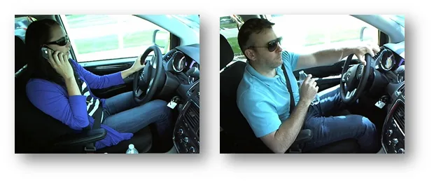
Figure 1. Images of common distractions while driving.

This makes the detection of these distractions essential to improve the road safety. Our aim was to explore ways to alert the driver; the prototype was not evaluated for its ability to prevent accidents. A validated tool could help reduce risk.

This project focuses on identifying common distractions, such as using a phone, looking in the mirror or drinking while driving.

Objective

The objective of this project is to adjust a model of Machine Learning capable of identify and classify different distractions while driving.

To do this, we will work with a technique of Deep Learning known as “Convolutional Neural Networks” (CNN or “Convolutional Neural Network”).

We will test some neural network architectures, all of them enhanced with pre-trained networks for image classification (transfer learning).

Image Set

The set of images that we have used in the framework of this project comes from a contest launched on the platform kaggle in 2016 (click here to see it).

All images have been obtained through a camera installed inside the car, always with a driver inside and in various everyday situations.

The photos have been taken in a controlled environment: a truck dragged the car through the streets, so that the drivers did not have to really drive.

To train the models, we have had a total of 22,424 images, classified into 10 categories:

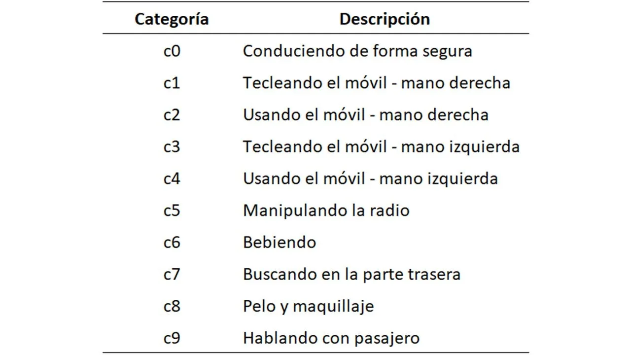
Figure 2. Description of the 10 categories of the experiment.

Exploratory Data Analysis

During Exploratory Data Analysis, we checked that every image had the same dimensions: (480, 640, 3).

In the random sample we reviewed, images appeared well classified across the ten categories. This spot check does not rule out errors elsewhere in the dataset from kaggle.

Images were also reasonably balanced across the ten categories, which simplified the initial exploration and let us move on to training the cnn.

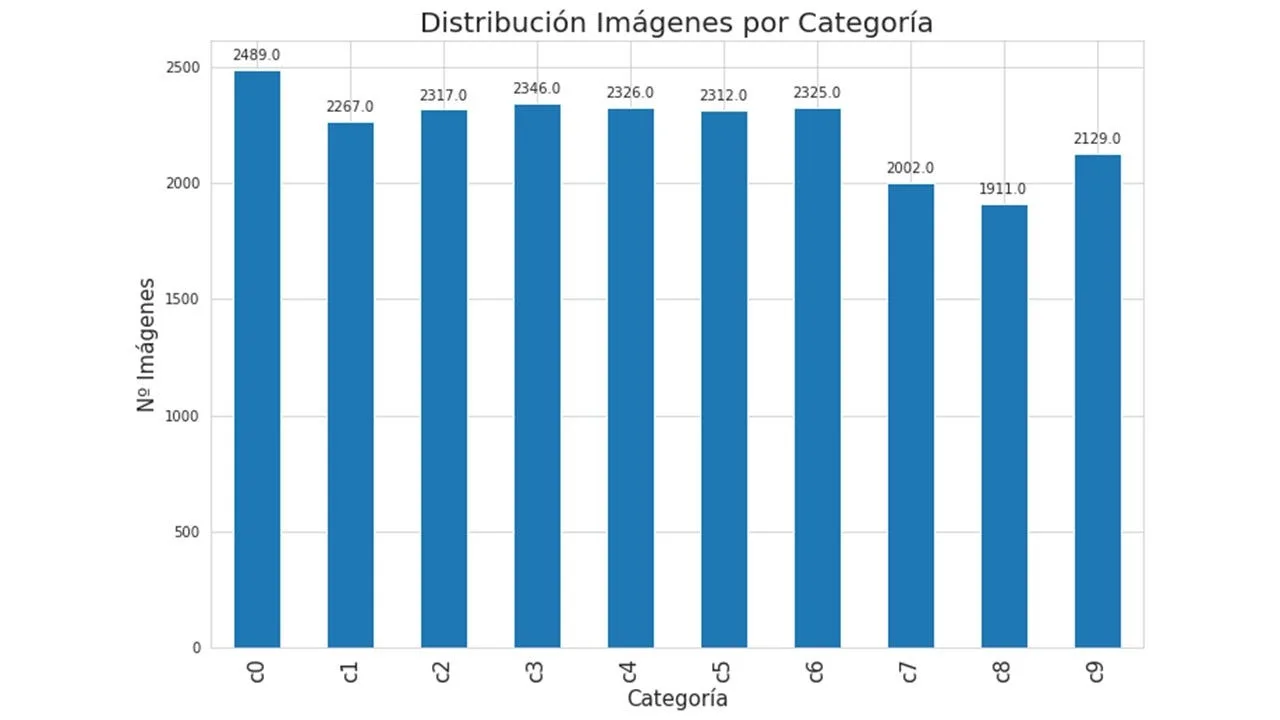
Figure 3. Distribution of the number of images among the 10 categories of the experiment.

The platform also provided kaggle 79,725 images for testing, without public labels.

It is important to mention that the training and testing images were divided into kaggle in such a way that the same driver did not appear in both sets (training and testing).

In general, the 10 categories could be considered “exclusive", except for the categories "c0” (driving safely) and “c9” (talking to passenger), which are more similar to each other and could be considered “not exclusive”, since, in some situations, they have in common the 2 hands placed on the steering wheel.

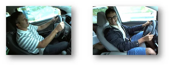
Figure 4. Images of 2 drivers, the first from the “c0” category, and the second, from the “c9” category.

Implementation

In general terms, we have followed the following steps to adjust the Convolutional Neural Networks presented in this project:

Download and pre-process driver images.
Build and train a model to classify driver images.
Check the fit of the model and improve it using different techniques.

Transfer Learning

Normally, there is no need to train a Convolutional Neural Network from scratch.

Training convolutional networks on large datasets such as ImageNet, can require substantial time and multiple GPUs. The cost depends on the model and hardware.

On the other hand, an increasingly common practice is the use of pre-trained networks as a fixed feature extractor, or as an initial network for finer adjustments.

The pre-trained network VGG appealed to us because of its simplicity and the results of previous work. We used its convolutional base as the starting point for our own classifier.

This lets VGG act as a feature extractor while we train our own classifier at the end of the network (top model).

In this project, we will use the pre-trained network “VGG16", as a starting point. For the most fine tuning, we will use three final layers, proposed in this link (“Hands-on Transfer Learning with Keras and the VGG16 Model”).

From the result of this first adjustment, we will build new models, with more layers. We will also use the resource of Data augmentation, and we will even dare to change the “VGG16” for the “VGG19", more complex pre-trained neural network, since it has 3 more layers than the "VGG16”.

Amazon Web Services

The adjustments of this first model and all the others presented in this article have been made in SageMaker of Amazon Web Services. For this, we have had the credit of 1.000$ that Amazon granted us for being part of the family Saturdays.AI.

We have chosen the computing center located in 'US East (Ohio)us-east-2', since this center had GPU machines. The machine chosen to open the instance of our notebook in SageMaker has been: 'ml.p3.2xlarge’.

Parameters and Evaluation of Models

A summary of the parameters of the fitted models will be presented below in table mode.

In any case, it is worth mentioning that, in all models, we have set batch = 32 and Epochs = 25, so that there was a basis of comparability between the model fits.

To evaluate the fitted models, in addition to the graphs of accuracy and of loss generated by the algorithm, we have classified 1,002 images, which from now on we will call 'Test Data’.

These images have been chosen randomly from the 79,725 images not classified for testing, with the aim of having a measure of accuracy on a set of images totally unrelated to the data used for training ('Test Data’ Accuracy).

We have also prepared a code in Google Colab (“model_test.ipynb”), in order to visualize the result of the model in each image, as you can see in the GIF below.

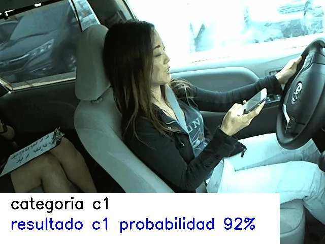
Figure 5. Output of “model_test.ipynb”.

Model 1: VGG16 + 3 Layers

As mentioned above, for the first model (“base”) we have used the pre-trained network “VGG16”, and for the finest adjustment, we have used three final layers.

The result of the adjustment of this model could be considered satisfactory, taking into account that this has been the first attempt at modeling the project:

‘Test Data’ Accuracy: 80,44%

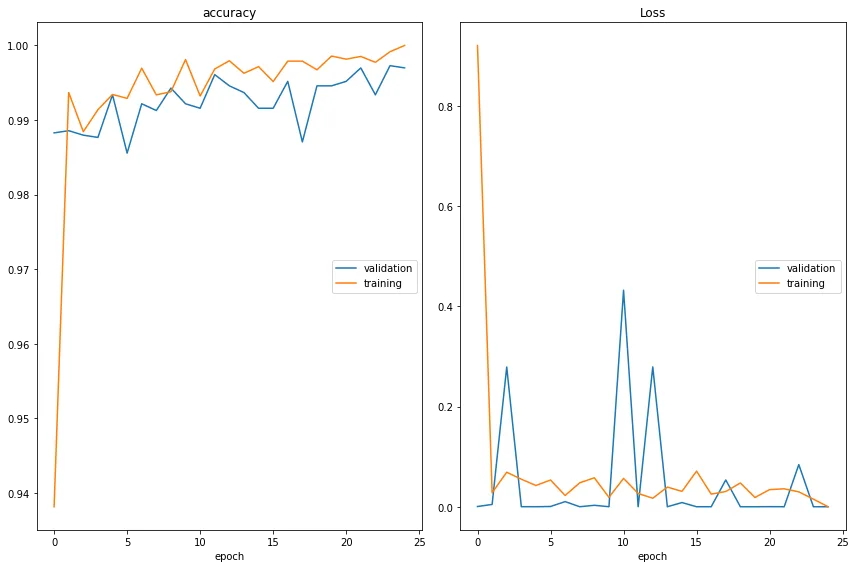
Figure 6. Accuracy and loss of Model 1.

Model 2: VGG16 + 3 Layers + Data augmentation

To improve the previous model, we have considered using the resource of “Data augmentation”.

At first, we did not know what some of the various parameters available to make the Data augmentation, or what their ranges meant.

To solve this, we did a series of tests, to be able to decide which parameters of Data augmentation we wanted to use in our set of images and their respective ranges.

Being a controlled experiment, the set of images used required a Data augmentation controlled and modest, taking into account that exaggerated changes applied to the original images could be counterproductive.

For example, we have decided not to do “rotations”, since we ran the risk of generating “unnatural” images.

The parameters of Data augmentation that we have used have been: “zoom”, “width”, “height” and “brightness”. Here are some examples.

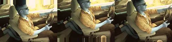
Figure 7. Zoom_range = [0.95, 1.05]

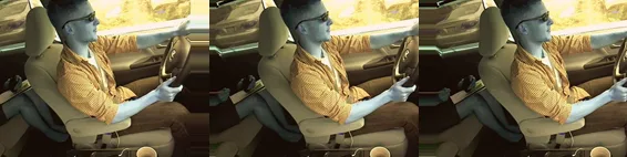
Figure 8. width_shift_range = 0.1

Note: The images have that tone due to RGB preprocessing.

The result of the adjustment of this model has improved considerably compared to the previous one (Model 1), so we have decided to continue using Data augmentation in the following models adjusted within the framework of this project.

‘Test Data’ Accuracy: 83,73%

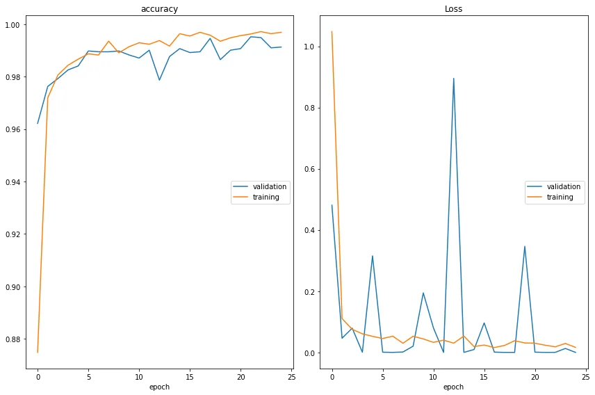
Figure 9. Accuracy and loss of Model 2.

Model 3: VGG16 + 5 Layers + Data augmentation

To improve the previous model, we added 2 layers to the final neural network (top model), maintaining the same parameters of Data augmentation of the previous model.

A significant improvement is observed in the accuracy of the model in 'Test Data’:

‘Test Data’ Accuracy: 88,12%

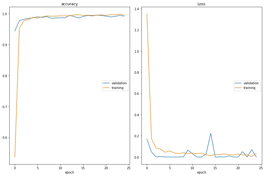
Figure 10. Accuracy and loss of Model 3.

Model 4: VGG19 + 5 Layers + Data augmentation

After improving the results, we decided to try a different pretrained network, to continue exploring new paths towards improvement.

We have used the network “VGG19", which contains three more layers than the network “VGG16”.

In this case, the results of accuracy did not improve on Model 3:

‘Test Data’ Accuracy: 84,53%

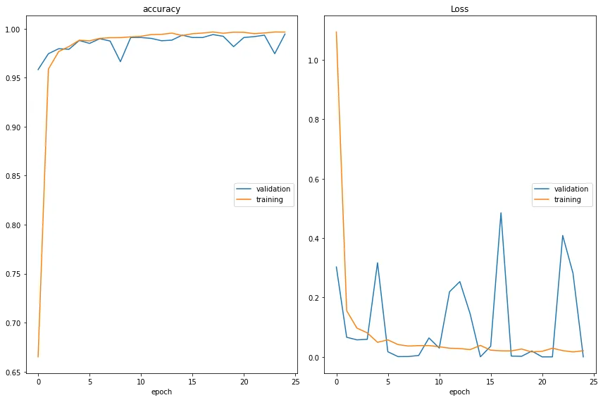
Figure 11. Accuracy and loss of Model 4.

So we have decided to use the network again “VGG16” for the adjustment of the following model.

Model 5: VGG16 + 9 Layers + Data augmentation

To continue exploring other possible improvements regarding the accuracy of the model, we have decided considerably increase the number of layers, from 5 a 9, maintaining the Data augmentation previous.

In this case, we have not improved the accuracy regarding the Model 3, although the result has been quite acceptable:

‘Test Data’ Accuracy: 86,63%

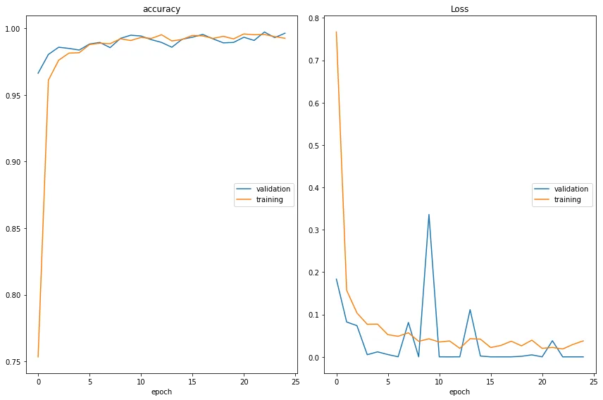
Figure 12. Accuracy and loss of Model 5.

Summary Table

The table below details the 5 adjusted models and the line of reasoning followed to adjust them, step by step.

In blue, the changes implemented from the first model (“base”), and the best results of accuracy (> 85%).

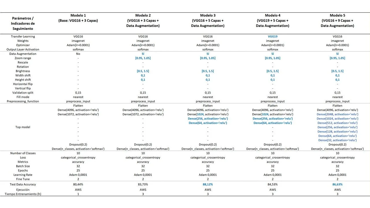
Figure 13. Parameters and results of the 5 adjusted models.

Confusion Matrix: Model 3

The per-class accuracy results for Model 3 were generally satisfactory.

This is reflected in the Confusion Matrix of the model.

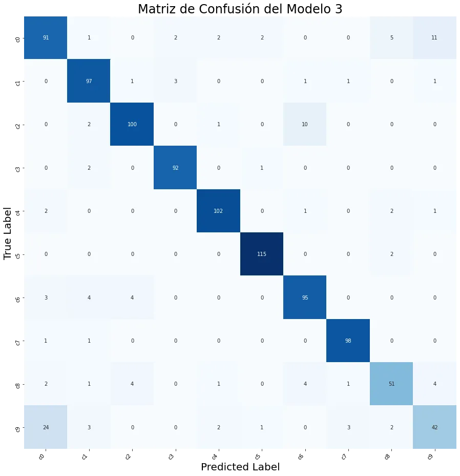
Figure 14. Model 3 Confusion Matrix.

The following categories stand out for their high success rate (>95%): “c3” (typing mobile phone - left hand), “c5” (manipulating the radio) and “c7” (looking in the back).

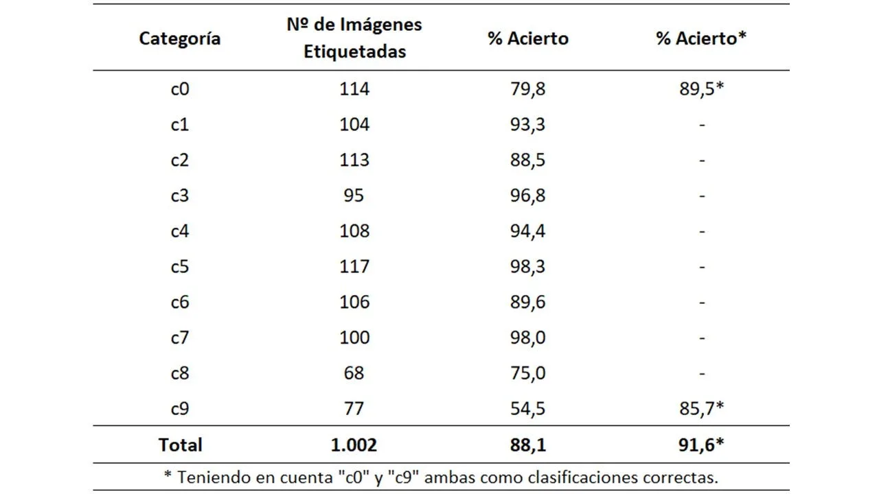
Figure 15. Correct percentages by category.

Accuracy drops notably for category “c9” (talking to passenger). This happens because the categories “c0” and “c9” could be considered the “less exclusive”, as mentioned previously.

If we accepted both c0 and c9 for images labelled c9, accuracy for that class would rise from 54.5% to 85.7%, an increase of 31.2 percentage points. This exploratory calculation changes the evaluation criterion; it is not a model improvement or a metric comparable with the original accuracy.

We have carried out this calculation to try to quantify the impact on accuracy for the fact of having worked with a couple of categories “somewhat less exclusive”.

A clearer distinction between c0 and c9 could help with labelling and evaluation. Any performance improvement would still need to be checked on an independent dataset. Repeatedly comparing models on the same 1,002 images makes that set part of model selection rather than an independent final test.

On the other hand, we understand that the study has to reflect everyday situations, since they will be the reality to be faced when deploying any model in real life.

Conclusions

The great computational capacity required by these models meant we spent a substantial part of the project resolving code execution problems.

We have had to learn to use the services of Amazon Web Services to make it viable, and the models of this project have been able to be trained thanks to the GPUs available from this platform.

Below are some conclusions and lessons learned after developing this project:

Adding more layers to a neural network does not always improve accuracy model fit. This fact has been seen in the adjustments of Models 3 and 5.
The resource of Data augmentation must be used with judgment, after an analysis of the initial set of images, since its indiscriminate use can be counterproductive.
The teamwork was fundamental. The varied backgrounds of our team and the coordinators at Saturdays.AI Donostia gave us a broad and enriching vision.

The road has not been easy and has required many hours of training. But believe us:it has been worth it!

Next Steps

As next steps, we consider the following:

Train a second, more specialised model to distinguish between categories “c0” and “c9”.
Retrain the Model 4 (VGG19 + 5 layers + Data augmentation), but now with more “epochs". The idea is to observe if with more training the network "VGG19"converges to the same results observed with the network"VGG16”.
Run the Model 3 in one Jetson Nano Nvidia, and evaluate the model with a camera in a controlled setting before considering use while actually driving.

Work Team

And to say goodbye, we would like to introduce ourselves.

Hello. my name is Imanol Areizaga and I am an Industrial Engineer. Since my first work experiences I have been working on digitalization processes in the industrial field. On the way to Data Science you discover new horizons step by step and in this step that I am taking together with Saturdays.AI I am interested in how to apply Deep Learning in industry, a demanding field where reliability requirements depend on the application.

Hello everyone. my name is Henry Corazza Sef and I'm a statistician. Although I have chosen to work on the implementation of the 6 Sigma Methodology in the industrial area, I am still very interested in Data Science in general. After this course, I discovered another passion: the fascinating world of neural networks!

We thank the mentors and organizers of Saturdays.AI Donostia, especially to Beñat Galdós, Joxemari Gallastegi and Imanol Echeverria, for their professionalism, dedication and enthusiasm.

Repository

In the following repository you will find the code used to develop this application: https://github.com/SaturdaysAI/Projects/tree/master/Donostia/Donostia2021/focusondriving-main

More artificial intelligence!

Saturdays.AI makes AI more accessible through shared learning and projects with a social purpose. Our motto is AI4ALL IS AI4GOOD.

Explore the available courses

Meet the Saturdays.AI community