MaMamIA: supporting breast cancer diagnosis with machine learning

Zaragoza. First Edition. 2022

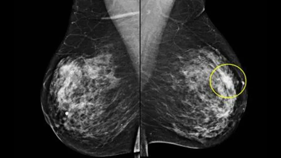
Breast cancer is a major cause of cancer deaths among women. It should not be described as the leading cause of all deaths in women. Timely detection and access to diagnosis and treatment are essential to reducing its impact.

Breast cancer is the most prevalent among women. It is estimated that The prevalence in Spain in 2020 is 516,827 people, according to REDECAN.

Breast cancer generally starts in the cells of the lobules, which are the milk-producing glands, or in the ducts, which are the pathways that transport milk from the lobules to the nipple.

Despite the progressive increase in survival from breast cancer, improving mortality rates from the disease is a medical and social need, since it has been studied that a 30% of the diagnosed patients will have a relapse of the disease. Likewise, breast cancer also affects men, being more deadly due to the scarcity of breast tissue, so it spreads to other organs more easily.

Breast cancer is the most common malignant tumor in women and the risk of suffering from it increases with age, with maximum incidence after the age of 50. Screening for this cancer through mammography, which is carried out among the population between 50 and 70 years old, allows reducing mortality. The 5.4 per thousand of the patients screened are positive. An early diagnosis of these cases is essential to carry out correct and effective treatment.

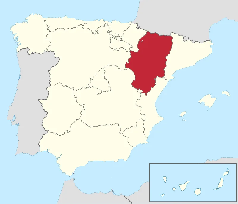
Fig. 3 — Map of Aragon [Wikipedia]

last year 800 new cancers breast cancer were detected only in the community of Aragon.

The current trend is towards an increase in cases not only due to less healthy lifestyle habits, but is also linked to the increase in the population in the detection program due to the arrival of boomers, as we can see in the following graph. So, the possibility of there being a large increase in cases in these years is quite high.

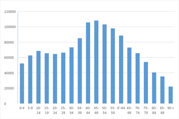
Fig. 4 — Distribution of target population by age

As a consequence of all of the above, we see a real need for the existence of some tool that helps with this problem of cancer detection. This is why, encouraged by the Saturdays AI project, we began addressing this problem through the application of Machine Learning and subsequent development of a tool (Mama Mia) for predicting the diagnosis of Breast Cancer.

Fig. 5 — Saturdays AI Emblem

This is a solution that aligns perfectly with SDG 3: Sustainable Development Goal Health and Wellbeing.

Fig. 6 — SDG 3

Likewise with SDG 10 on Reducing Inequalities, since it is in lower-income areas where more deaths are recorded. The use of all the work done here is released.

Fig. 7 — SDG 10

How are we going to do it?

Like any process in which you want to implement technology in a business, a methodology is necessary. We will not reinvent the wheel, we will use the iterative CRISP-DM methodology (Cross Industry Standard Process for Data Mining) that provides us with a guide structured in six phases, some of which are bidirectional, allowing us to return to a previous phase to review it.

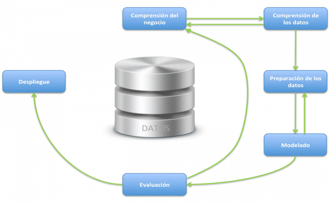
Fig. 8 — CRISP-DM methodology diagram [Google Images]

Phase 1 — Business Understanding

The objective of this project is the development of a tool for the prediction of breast cancer. For which we have the dataset of

https://archive.ics.uci.edu/ml/datasets/breast+cancer+wisconsin+(diagnostic)

Obtained from a digitized image of a fine needle aspirate (FNA) of a breast mass, they describe the characteristics of the cell nuclei present in the image.

Phase 2 — Data Understanding

We have started the project by seeing what data we specifically have. After obtaining our data from ICU and going into detail, our database is made up of 31 useful variables that we can break down into the diagnostic variable (if it is positive or negative) and 10 parameters that define the cells are given under 3 situations: the average value, the standard deviation and the worst case.

• Radio
• Texture: Standard deviation of grayscale values
• Perimeter
• Area
• Uniformity: Local variation in diameters
• Compactness: Perimeter²/area — 1
• Concavity: Severity of the concave points of the contour.
• Concave points: Number of concave points on the contour
• Symmetry
• Fractal dimension: approximation to a perfect sphere, which corresponds to 1.

These 30 variables are obtained from the analysis of the biopsy.

Within our data we have 213 malignant cases and 357 benign cases.

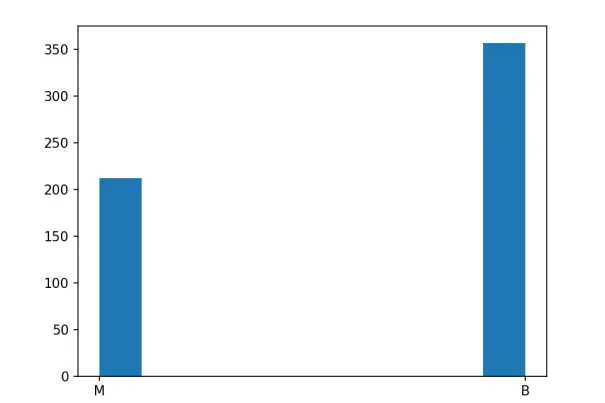
Fig. 9 — Diagnostic histogram

Phase 3 — Data preparing

Apart from the 31 useful variables, we find a column with NaN values that we eliminate along with the ID (identifier) of each case since it does not provide any information for prediction and we replace the diagnostic data: M and B with binary numerical values: 1 and 0.

So the first thing was to see what type of data we had: all floating point numbers except the diagnosis. Analyzing the data we can see that we do not have NaN values and they have the following statistical data:

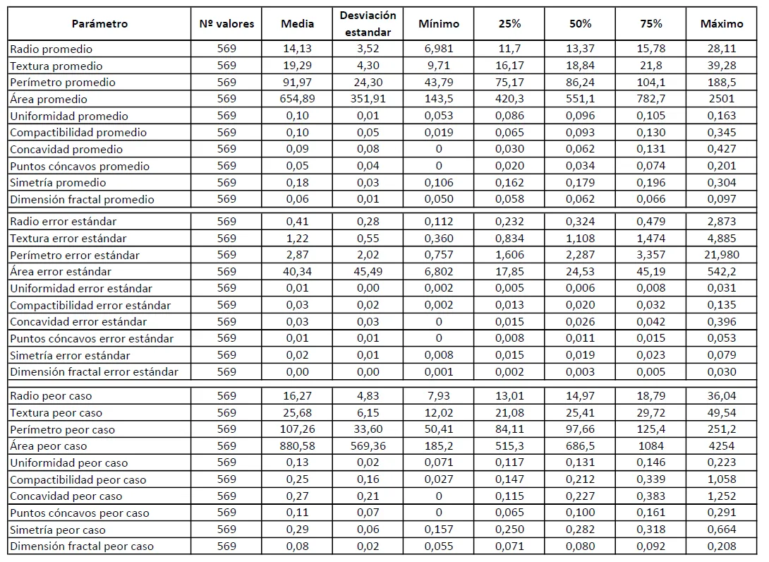
Table 0 — Data statistics

We have obtained the correlation graph using a heat map to see how the variables relate to each other and in our case the relationship with the one that matters most to us: the diagnosis ('diagnosis’).

We can see in the first row how there are parameters with a high direct correlation (light colors) and parameters with a slight inverse correlation (dark colors).

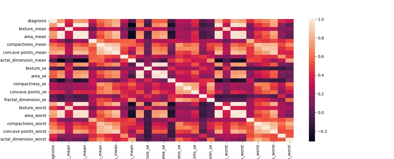
Fig. 10 — Variable correlation map

Now we are going to compare all the variables using box plots, separating for each variable the malignant cases (in red) and the benign cases (in green). These graphs help us to be able to identify some key variables. These will be those in which the distribution of malignant and benign is very different.

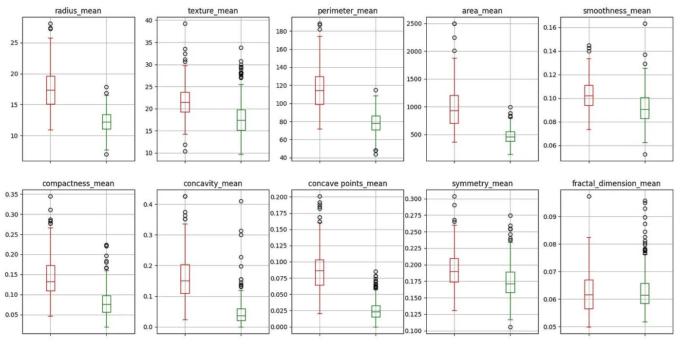
Fig. 11 — Boxplots of malignant and benign cases (average)

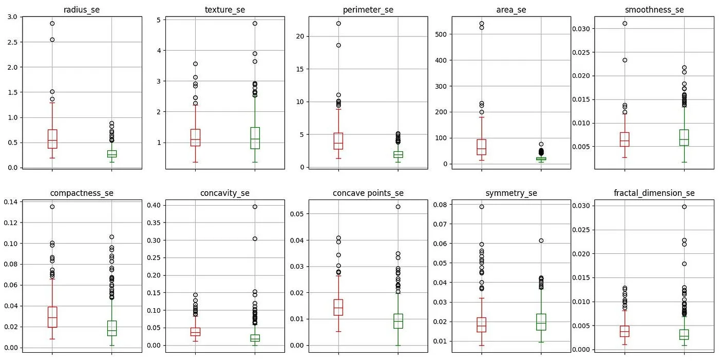
Fig. 12 — Boxplots of malignant and benign cases (standard deviation)

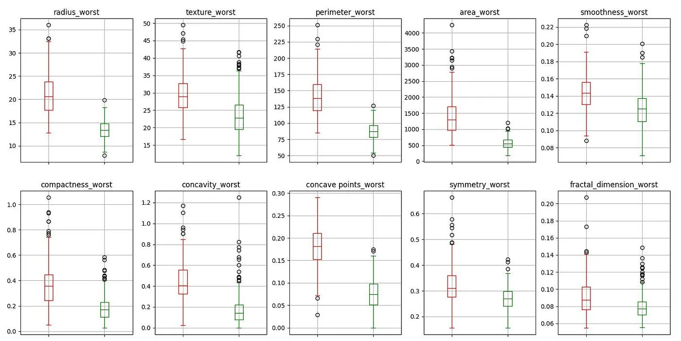
Fig. 13 — Boxplots of malignant and benign cases (worst cases)

We see that outliers occur quite frequently, usually above. This variability is possible since data in medical studies tends to be more variable than what we can find in other databases.

Before moving on to modeling we must normalize the variables to make better quality predictions.

Phase 4 and 5 — Modeling and evaluation

Given the typology of data we have, we have used supervised models (the data is labeled) and classification models (predicts a category). The models we have evaluated are:

• Logistic regression
• decision tree
• Random forest
• extra tree
• Super Vector Machine (SVM)
• Gradient Boosting
• K — nearest neighbors (KNN)
• MLP classification

In these models we have tested with random state 2. To do this, before introducing them into the model, we have separated the data with a ratio of 70–30 in training and evaluation respectively.

After evaluating these models we have obtained the following results:

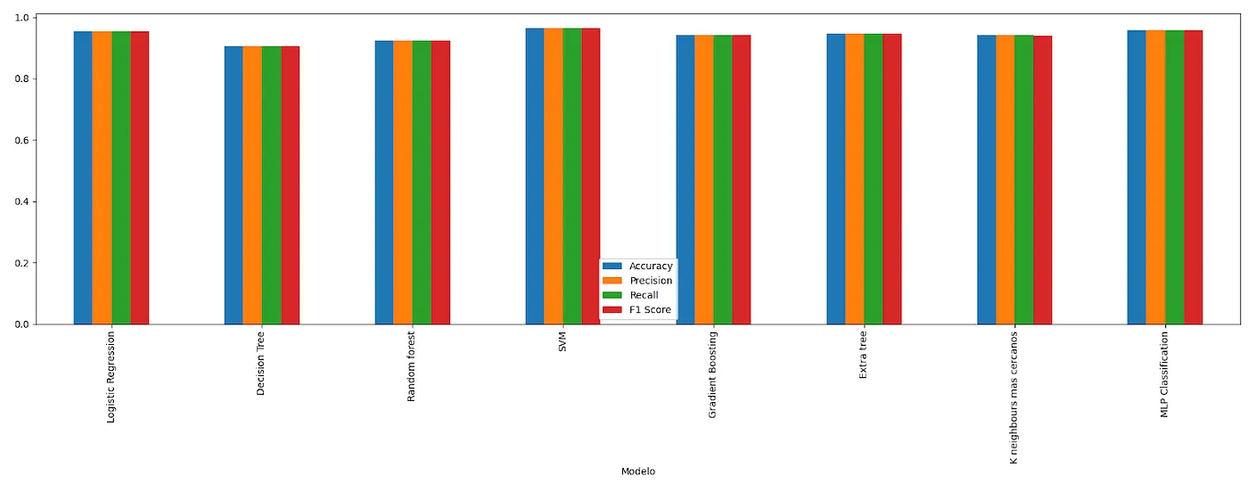
Fig. 14 — Metrics for all models

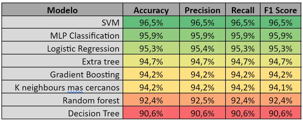
Table 1 — Model metrics

We can see how we obtain accuracy values (accuracy), precision (precision), Recall and F-score More than 90%. Models with a F-score greater than 95% are those that stand out for the best models in the face of the following stages, not without first checking several elements of the model.

It is a model with a high number of characteristics, so we ask ourselves several questions: Could a result be achieved with fewer variables? Are there dependencies between these? Are the results always good or was it a coincidence of the random state?

To do this, we begin to observe the importance of the variables (in cases that allow us to do so).

Influence variables

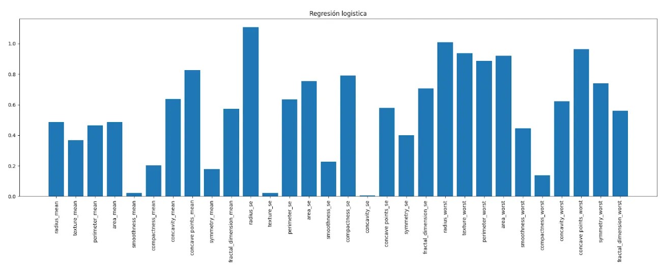
Fig. 15—Influence variables Logistic regression

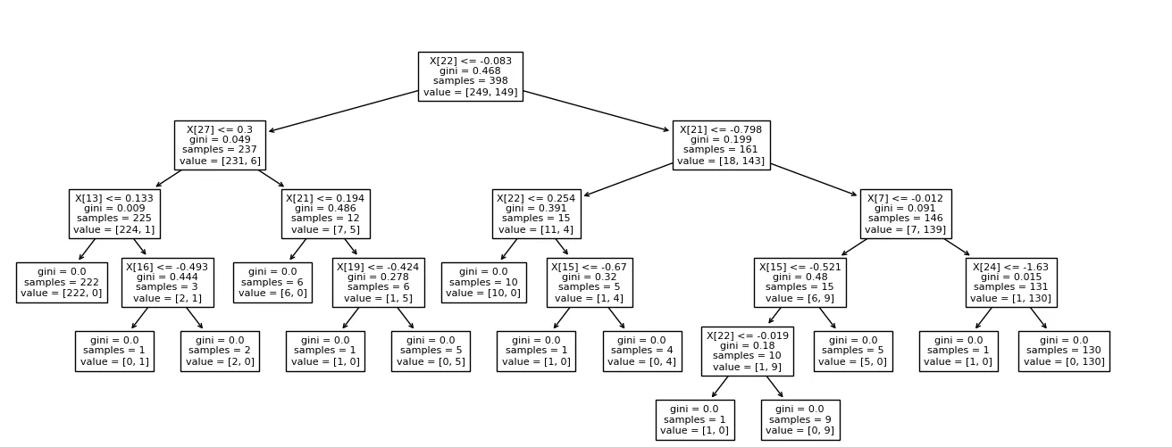
Fig 16. — Decision diagram of the Decision Tree

In the case of the decision tree (Decision tree) we can see according to which variables it is classifying.

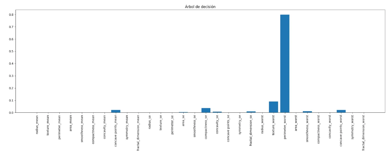
Fig. 17 — Decision Tree influence variables

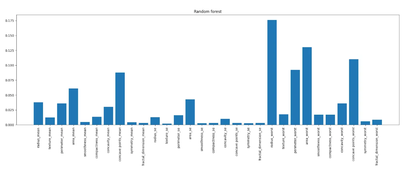
Fig. 18 — Random forest influence variables

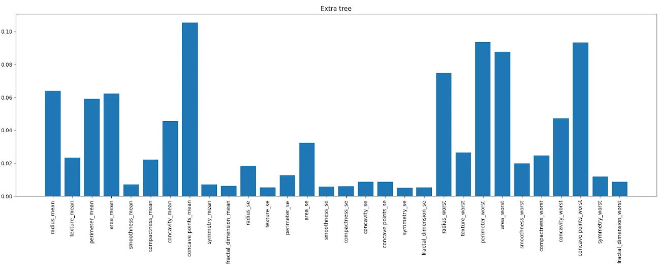
Fig. 19— Extra tree influence variables

Variable reduction and new metrics

Based on the importance of the variables that we have seen, we have chosen 3 combinations to simulate: with 10, 16 or all the variables. Chosen like this:

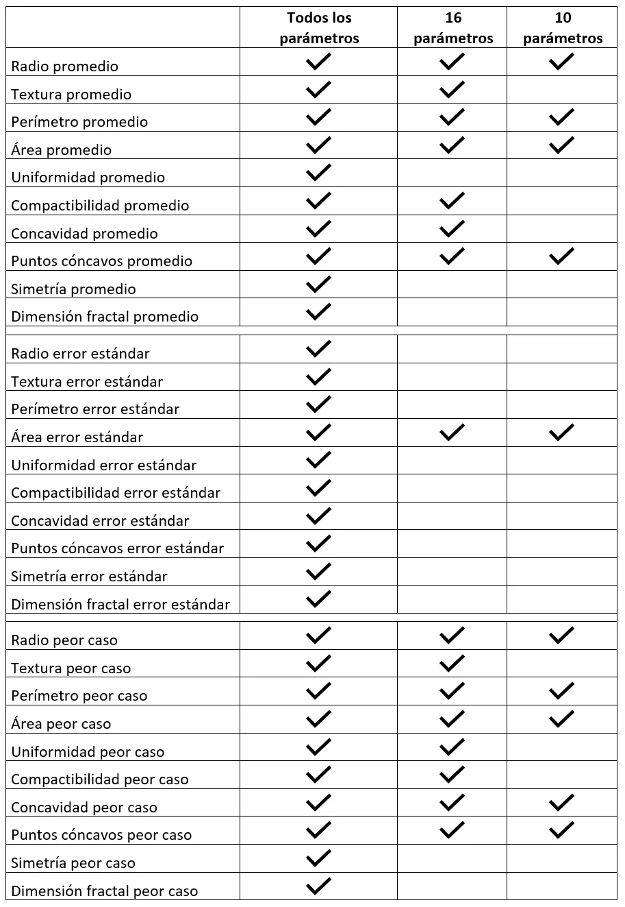
Table 2 — Model variables

The following results are obtained in the predictions for each of the 3 cases:

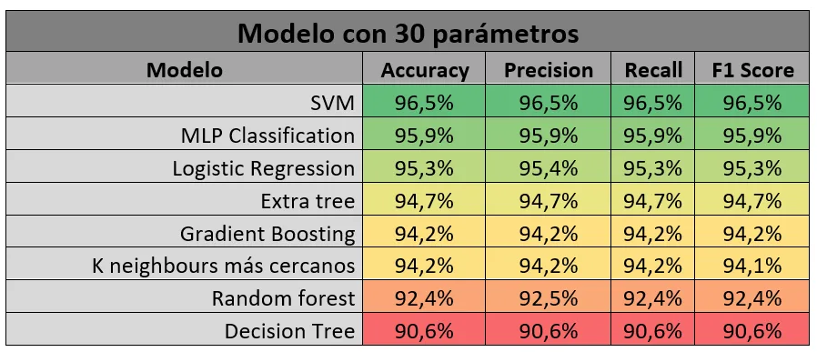
Table 3 — Model metrics 30 parameters

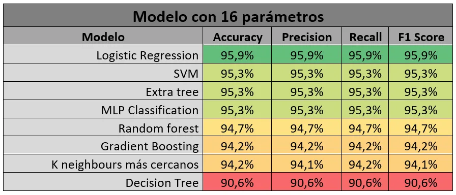
Table 4 — Model metrics 16 parameters

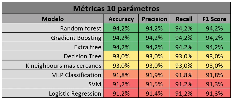
Table 5 — Metrics of the models 10 parameters

We set a selection criterion of a minimum F-score of 95%, therefore we chose a model with 16 parameters since it allows us to predict with sufficiently good metrics but with almost half as many parameters as the 30-parameter option.

After this we move on to see how its behavior is regarding the prediction of probabilities in relation to the seed effect. To do this we will look at the first 200 seeds, how they behave. To do this, we will make a histogram where we will accumulate the probabilities with which it predicts both for true positives and negatives, and for false negatives and positives.

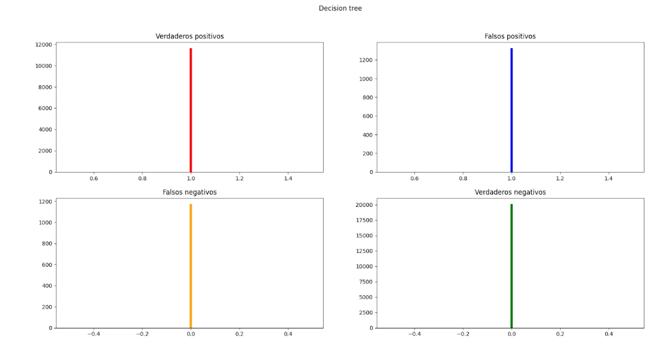
Fig. 210—Probability distribution Decision tree

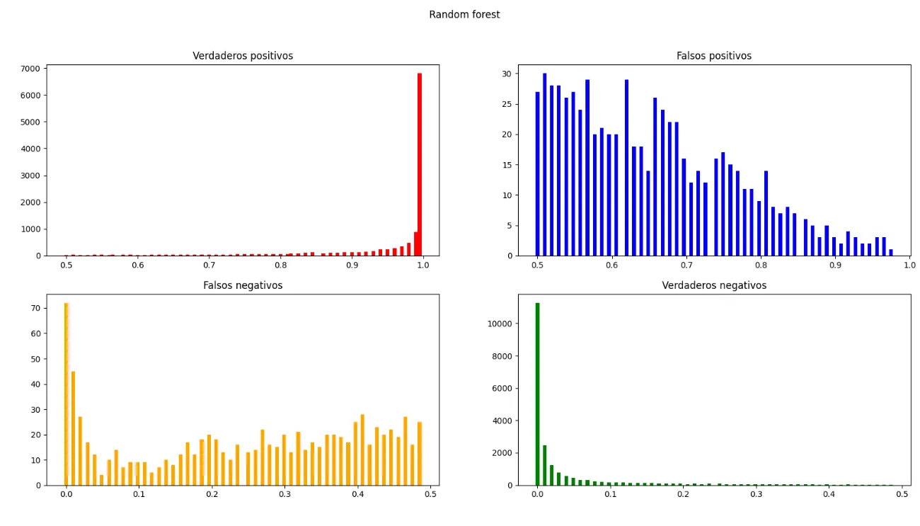
Fig. 21 — Random Forest probability distribution

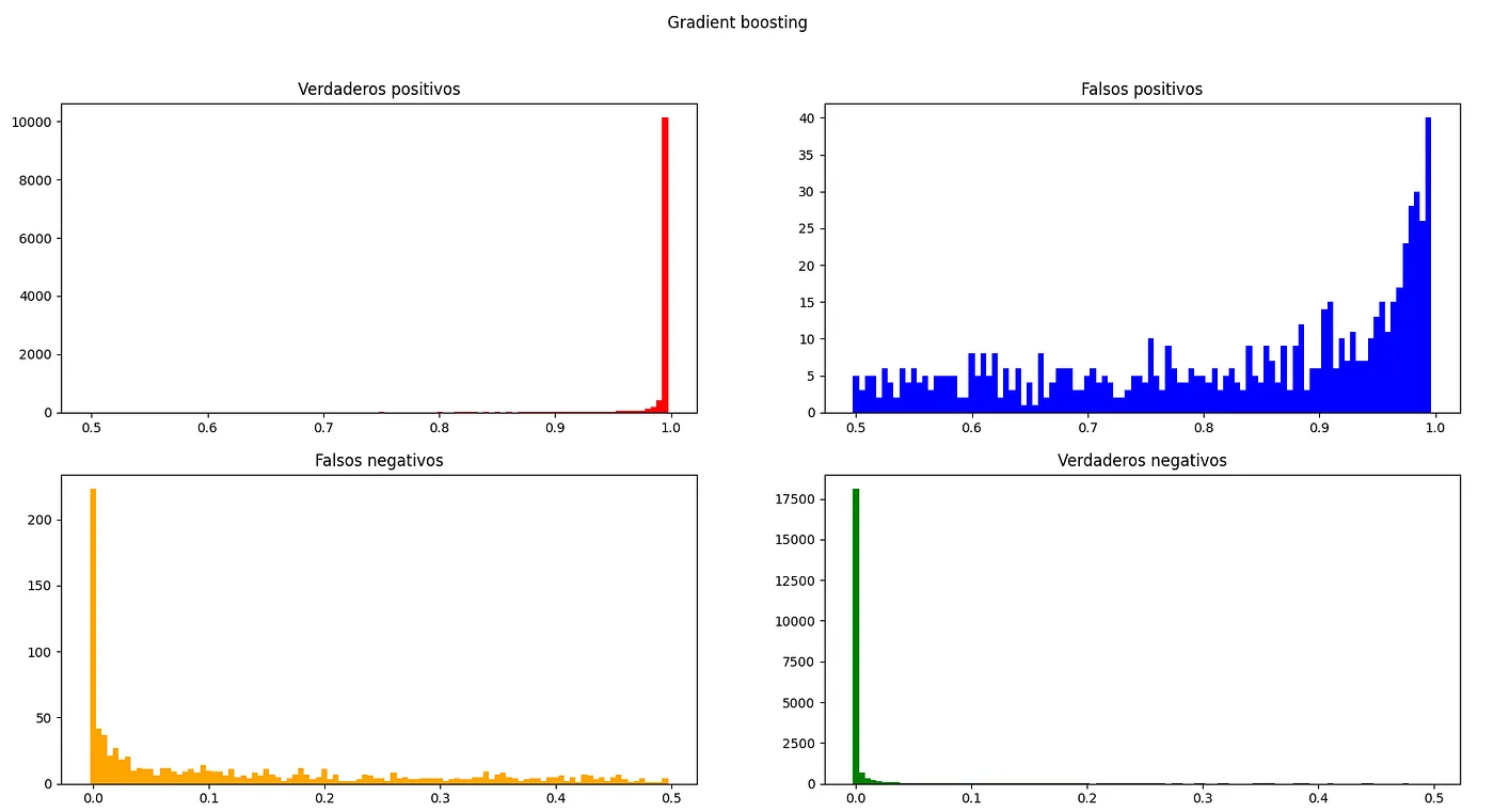
Fig. 22 — Gradient Boosting probability distribution

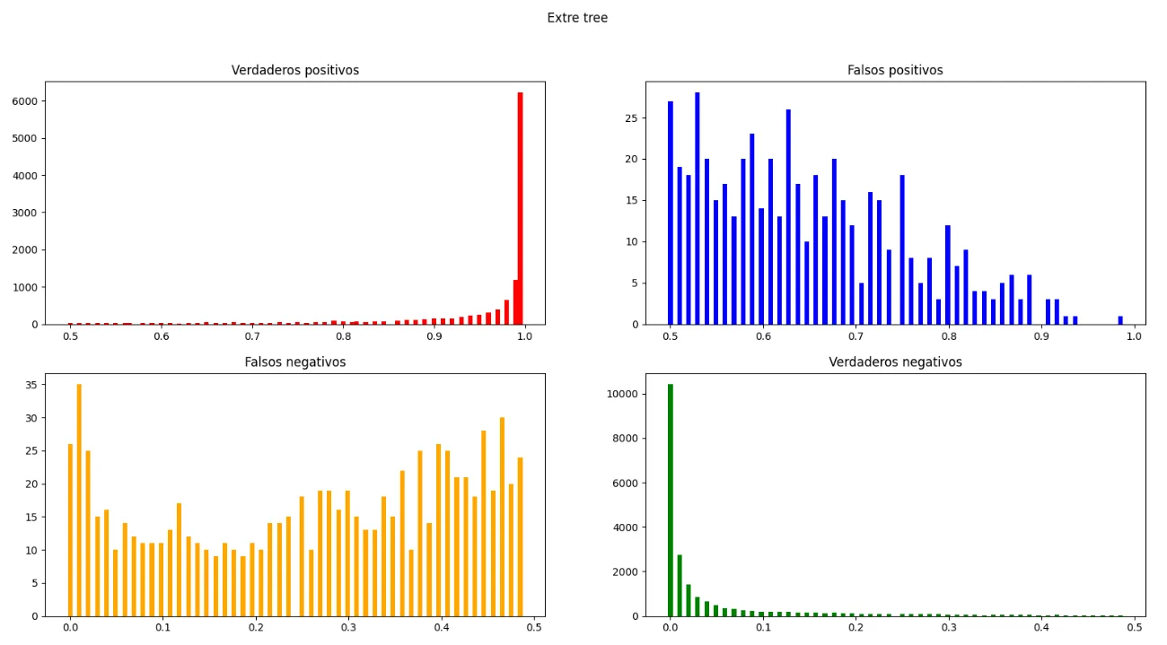
Fig. 23 — Extra tree probability distribution

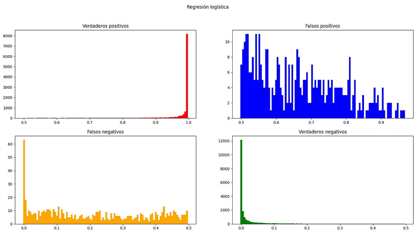
Fig. 24 — Probability distribution Logistic regression

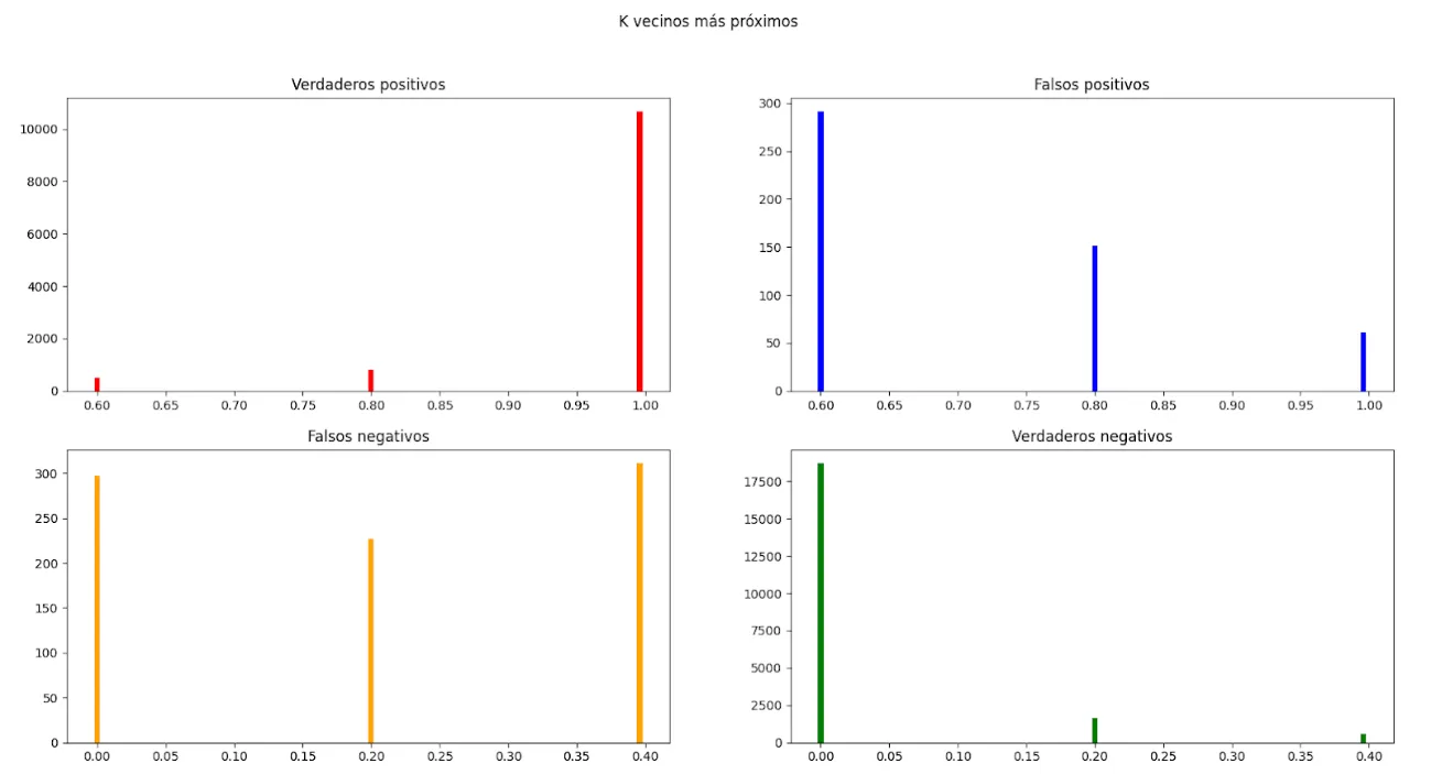
Fig. 25 — K nearest neighbors probability distribution

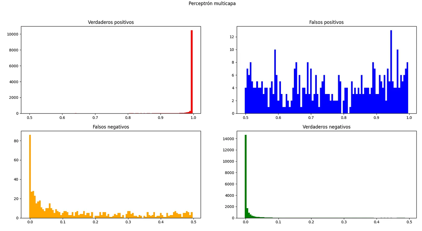
Fig. 26 — Multilayer Perceptron probability distribution

With all the simulations carried out we see how there are certain models that concentrate their values in higher and more concentrated metrics, these will be the ones we will choose.

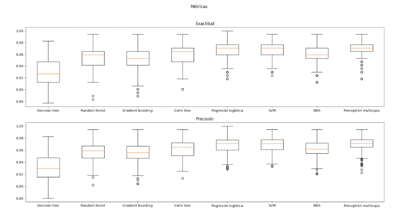
Fig. 27 — Accuracy and Precision of the models

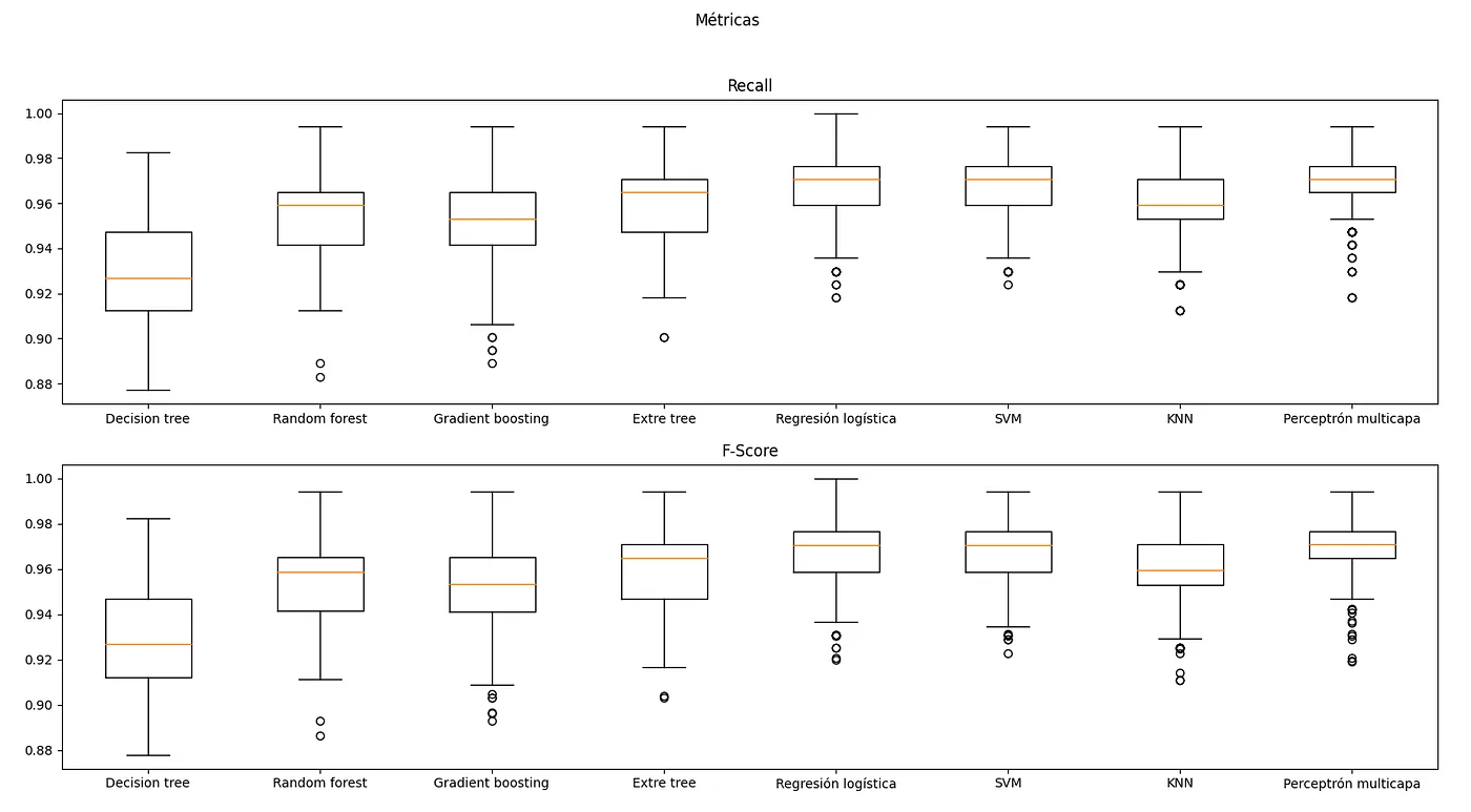
Fig. 28 - Recall and F-score of models

By only varying the initial random state, we achieve very high maximum metrics, classified in this table.

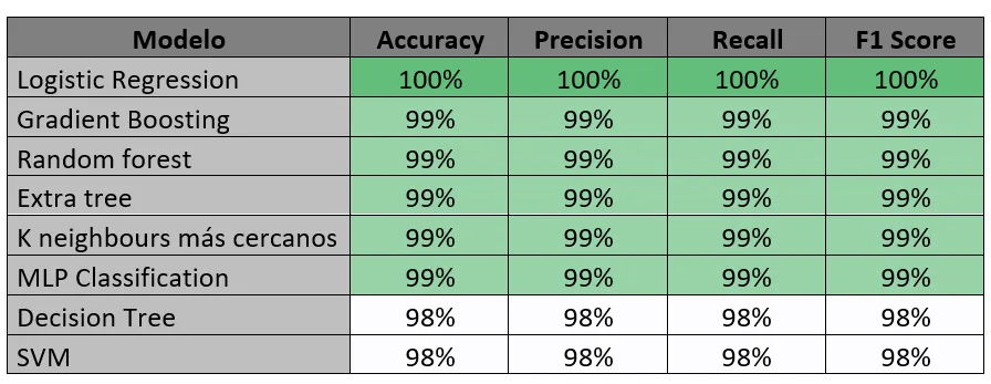
Table 6 — Maximum model metrics

Once we choose the best models (with higher and more concentrated F-score): SVM, Logistic Regression and MLP Classification (Multilayer Perceptron).

From now on we will try to achieve greater robustness by improving the 3 finalist models. To do this, we will test different combinations and once the model (or combination of final models) is selected, we will optimize it (if possible).

We have chosen the Logistic Regression, Support Vector Machine, and Multilayer Perceptron models. Since they have high metrics in a range that has varied less, so we assume better.

Assembly of various methods

Once we have very good models, one even with 100% metrics, we decided to combine them. Why combine them if they already have great metrics? So that it is more robust and more likely to get the result right in a case that has not been evaluated or trained.

Trying with Adaboosting and Bagging we obtain worse metrics.

And with voting we obtain slightly smaller values distributed like this:

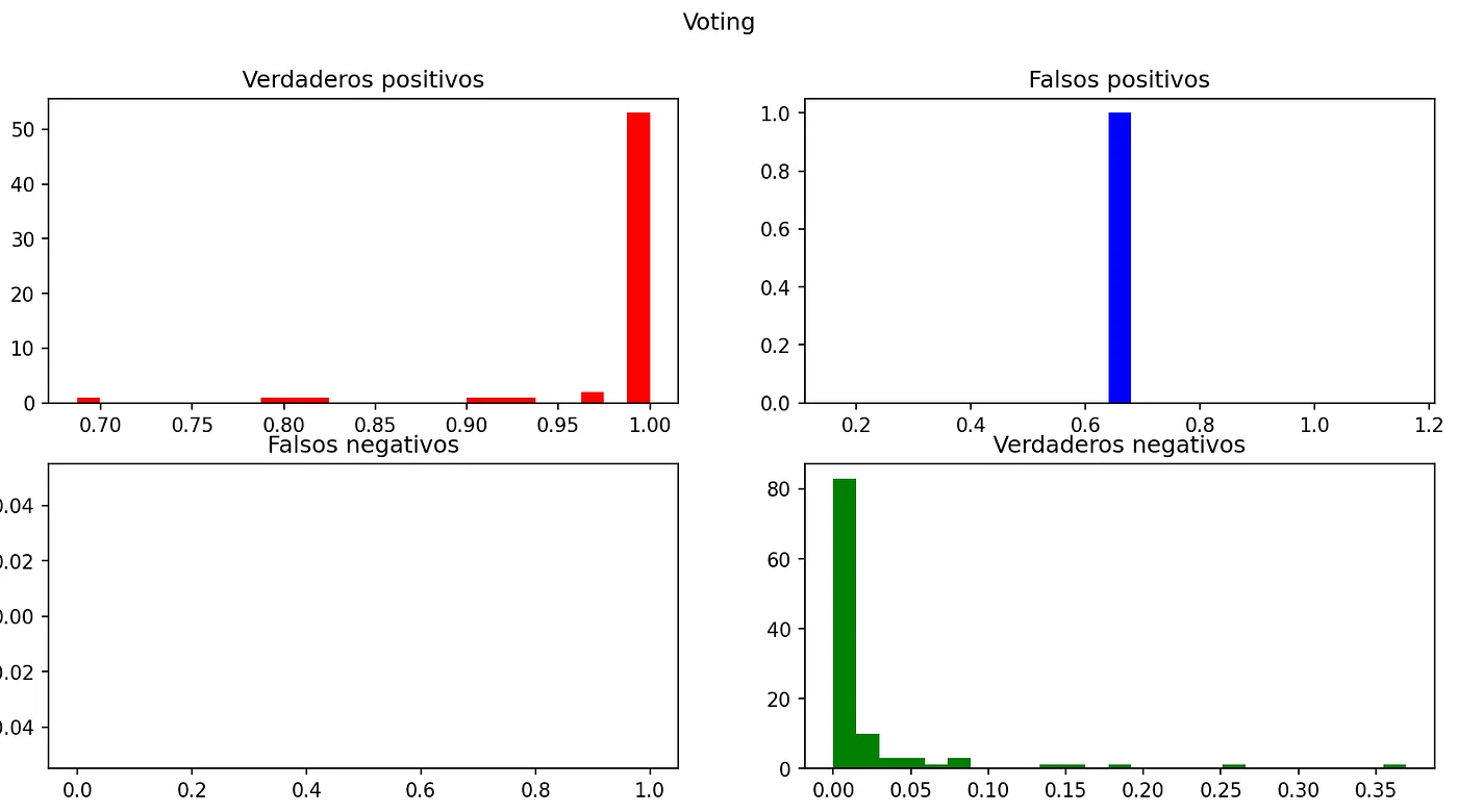
Fig. 29—Voting Probabilities

With metrics of:

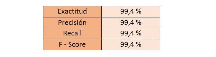
Table 7—Voting metrics

Model selection

Selecting the best seeds we obtain the following histograms:

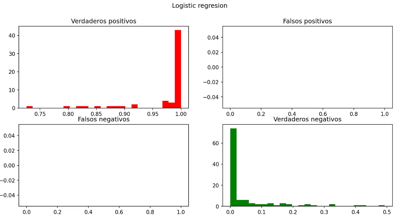
Fig. 30 — Probability Logistic Regression

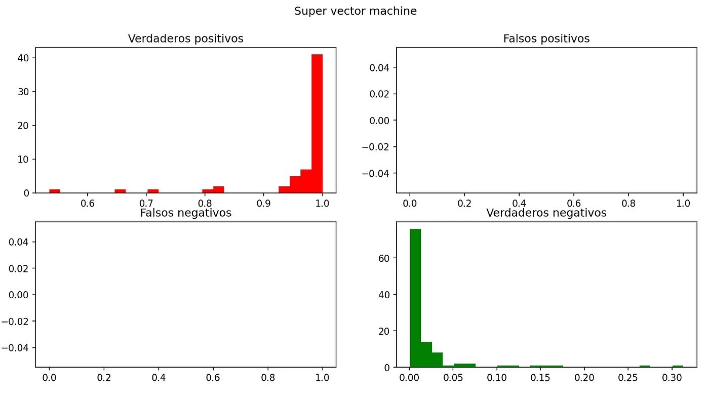
Fig. 31—Probability Super Vector Machine

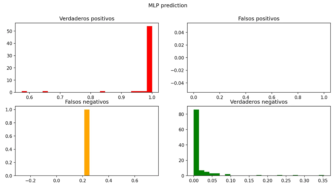
Fig. 32 — MLP Prediction Probability

We see how the MLP predicts with much higher probabilities, but with a false negative. The logistic regression stands out, which is correct in 100% of the cases. Here we can see the metrics of the models:

Table 8 — Metric comparison of the models

Hyperparameter tuning

We are going to use the Scikit-Learn library to adjust the hyperparameters of the algorithm in order to find which values would improve the data previously obtained.

We use GridSearchCV with the following values:

• Kernel: linear, poly, rbf and sigmoid
• C: 1000, 10, 1 and 0.01
• Gamma: 0.001 and 0.001

Obtaining the best results of 97.11%, with C equal to 1, gamma equal to 0.001 and linear kernel.

We did not get any significant improvement to the default parameters.

Final results

We choose logistic regression since it is the one that has had the best results and we have preferred it to voting since we cannot guarantee that with voting we will obtain a more robust system.

Phase 6 — Deployment

Once the model has been chosen and adjusted, to avoid doing the process again, it is saved through the library joblib thus being able to use it later. To provide the project with great accessibility we decided to publish a website that uses the model, for which we resorted to the open-source library: streamlit, which allows us in a simple way to create a simple web application that uses said model.

It is only necessary to create a data collection form to fill out and when you send the form, the website normalizes and scales the data according to the data with which the model has been trained to pass it to it and make the prediction.

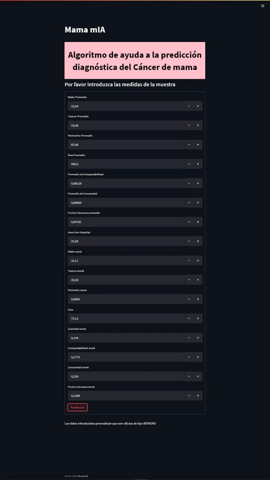
Fig. 33 — Main screen of the MaMamIA application

Next steps

• Complement the prediction of breast cancer diagnosis with the prediction of cancer recurrence.
• Development of an application with the option of introducing a different number of variables depending on the precision sought.
• Implementation of prediction using photographs.

Members

• Victor Villanova (vvb.curioso@gmail.com)

Student of the joint program in master's degree in Industrial Engineering and master's degree in Renewable Energy and Energy Efficiency. Passionate about the unknown and nature, handyman and scout.

• Miguel E. Calvo (mecalvon@gmail.com)

Currently Systems Management and IT Technician in HEALTH (Government of Aragon). Curious and restless technological.

Open video or resource

Repository

The code is available at https://github.com/gitmecalvon/mamamIA

More artificial intelligence!

The mission of Saturdays.ai is to make artificial intelligence more accessible (#ai4all) through intensive courses and programs where projects for good are carried out (#ai4good).

Explore our AI master’s programme at https://saturdays.ai/master-ia-online/

If you want to learn more about artificial intelligence join our community at community.saturdays.ai or visit us on our website www.saturdays.ai Join us!

WHO: breast cancer information