Analysis of Depression in Social Networks: An application in Biostatistics
Facemood explores social media use, mood and self-reported symptoms using statistical and machine learning methods.
A learning project shared by the community. The article documents its team, methods and results; it does not establish that the prototype is ready for real-world use.

Donostia. First Edition. 2020
Introduction
Have you ever wondered if using social media so much could affect your mood? There are those who relate misuse of social networks to psychological problems such as depression, but what is true in this idea? Is there scientific evidence that alerts us to real dangers of social networks, or are these fears unfounded?
During the first edition of the Saturdays AI program in Euskadi, the group Facemood set out to explore the relationship between social media use and symptoms associated with depression. We used statistical tools and Machine Learning that helped us understand the relationship between these variables.
The depression It constitutes a major public health problem, as it is a major risk factor for suicide, which claims hundreds of thousands of lives each year.
Understanding factors associated with depression can contribute to public policy and support efforts to save lives.
Who are we?
As if it were a futsal match, we present our starting quintet:
- Hello! I’m Sergio Navarro, and I work in software engineering. I’m a full stack developer at a small startup in Álava, spending my time among lines of code, databases and Stack Overflow questions that might help me solve the bug keeping me awake.
As a starting point, we rely on the work carried out by a group of Dutch and American researchers titled: ‘Social Media and Depression Symptoms: A Network Perspective’ (DOI:10.1037/xge0000528; also available as an open-access paper). The study examined temporal relationships between depressive symptoms and passive social media use, such as scrolling in the feed of news or photographs. These are observed associations, not experimental proof of causation.
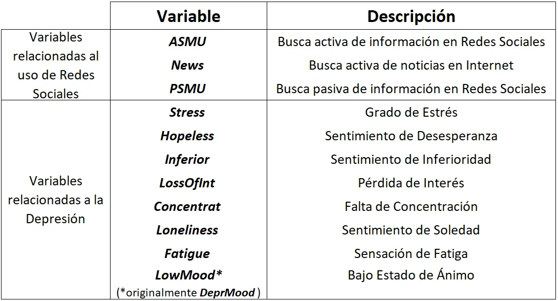
To obtain the data, each of the participants in the study received a questionnaire on their mobile phone in which they had to answer from 0 to 100 how they felt in reference to each of the possible symptoms of depression: lack of energy (Fatigue), low mood (LowMood), loneliness (Loneliness), concentration problems (Concentration), loss of interest (Loss of Interest), feeling of inferiority (Inferiority), hopelessness (Hopeless), and stress (Stress). They also had to answer from 0 to 100 to three questions related to the use of Social Networks: passive use (PSMU), active (ASMU), and news consultation (News: access information of a political nature or public interest). Participants filled out this questionnaire seven times a day for 14 days.
Below is a brief description of the 11 study variables:
To carry out this project, we have planned an analysis strategy according to the scheme below, in which we have used different methodologies and tools:
1. EDA (Exploratory Data Analysis)
2. Cluster Analysis
3. ANOVA of Repeated Measures
4. Regression Analysis
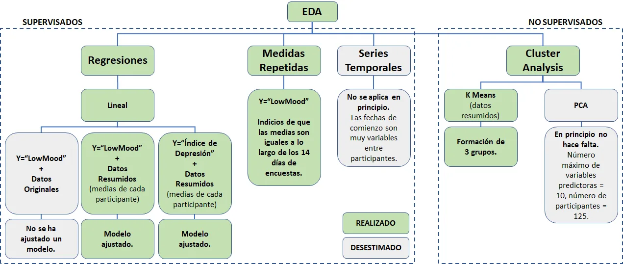
Figure 1. Analysis Strategy.
1. EDA (Exploratory Data Analysis)
The dataset comes from a scientific publication with documentation from the original study. This helps us understand its origin, but does not by itself guarantee better quality than a dataset obtained from a data-sharing platform open source like kaggle. In every case, we need to examine data quality, patterns and limitations before applying Machine Learning.
The first phase consisted of identifying those measurements that we consider valid. Logically, many of the participants forgot to carry out some of them (carrying out 7 measurements a day for 14 days is not an easy task. ?), or they didn't know how to respond to some of the symptoms (quantifying your mood from 0 to 100 isn't either...). All these measurements were eliminated.
In a second phase, we looked at whether the remaining measurements were coherent: they do not have the same value in all symptoms, they are not recurrent responses, they were carried out within the defined time period, etc.
In this way, we are ready to take action!
2. Cluster Analysis
The next phase consisted of carrying out a Cluster Analysis, one of the techniques of Machine Learning to identify groups in the dataset. We use the methods Elbow and Silhouette to get the number of clusters optimal and the algorithm K-means, technique unsupervised learning to do clustering.
Identification of the optimal number of clusters
Method Elbow: in this the average distortion of the clusters, that is, the average distance of the centroid to all points on the cluster. This is obtained with the algorithm K-means depending on the number of clusters. To solve this exercise, we have created the function plot_elbow, which receives a data set and a chart title. We set the values of the parameters max_k to 10 and tested values from 1 to 9, plotting the results.
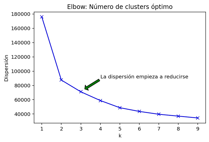
Figure 2. Graph representing the Elbow method.
The team interpreted the elbow curve as suggesting three clusters as a reasonable compromise. We checked this choice against the silhouette coefficient.
Silhouette method: for each observation, a is the mean distance to the other observations in its own cluster; b is the smallest mean distance to observations in another cluster. The coefficient is calculated as (b − a) / max(a, b) and ranges from −1 to 1.
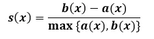
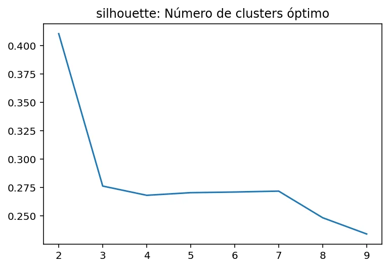
Figure 3. Graphic representing the Silhouette method.
With this method we verify that 3 can be a good value to test our cluster analysis.
Algorithm implementation k-means and visualization of the groups in a 3D graph
The algorithm receives a set of data to train it and a number of clusters to divide it. Through the method predict assigns each observation in the dataset to a cluster dataset, and finally each data is represented with a different color depending on the cluster to which it has been assigned. We can see the result in the Figure 4 and the distribution of participants in the Figure 5.
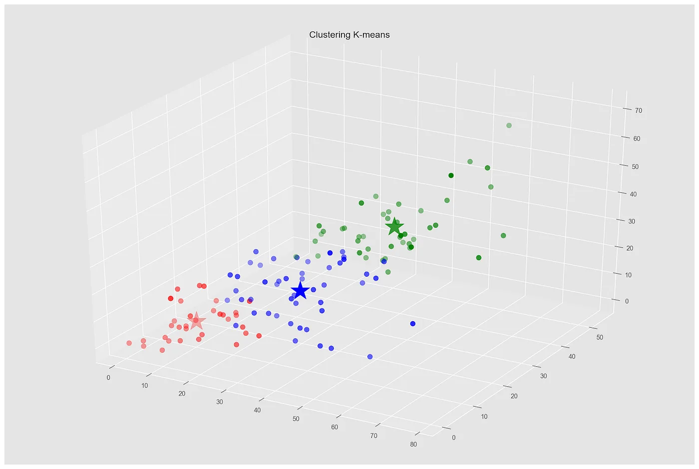
Figure 4. Visualization of the groups in a 3D graph.
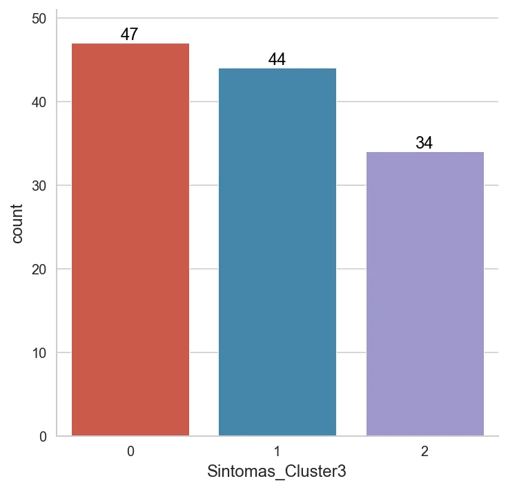
Figure 5. Distribution of participants by cluster.
Finally, to conclude with the Cluster Analysis, We have created a series of graphs (overlapping histograms) to identify at a glance the differences in each variable between the members of each cluster.
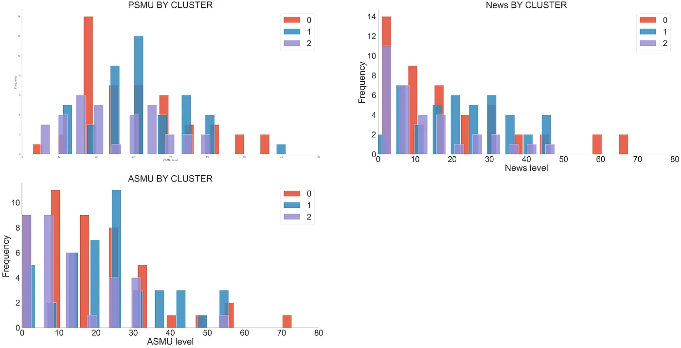
Figure 6. Social media variables by cluster.
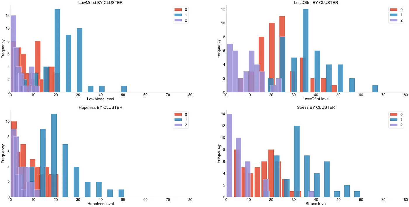
Figure 7. Variables related to depression, for cluster.
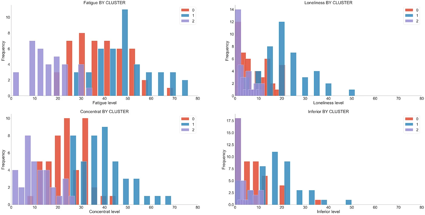
Figure 8. Variables related to depression, for cluster.
It is observed that the 3 clusters are different when it comes to symptoms related to depression, being the Cluster 1 the one that contains the higher average scores across the eight self-reported symptoms. This describes differences in questionnaire responses, not a diagnosis of depression.
However, as we can see in the Figure 6 (RR.SS variables. by Cluster), in the case of variables related to RR.SS. We did not find major differences between clusters.

Figure 9. Table of averages by cluster.
3. ANOVA of Repeated Measures
There are two aspects to this dataset that especially caught our attention. On the one hand, the fact of having taken measurements for two weeks offers us the possibility of exploring whether these measurements vary over time. Using a line graph or lineplot shows how each measured symptom varies on average.
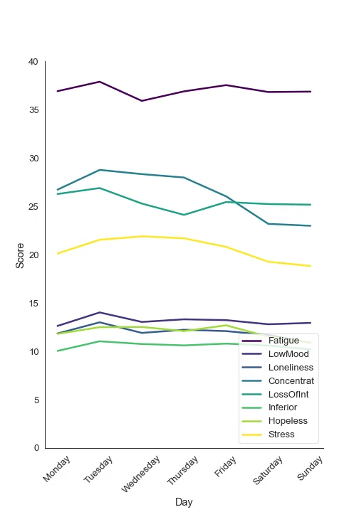
Figure 10. Means of each variable grouped by day of the week.
Although there appears to be some variation over time in some of the variables, we cannot be sure at a glance whether the data would be expected to vary this way by pure chance or because we have not used a very good measuring instrument.
On the other hand, we know that a large number of measurements were carried out on each participant. As we explained above, 125 subjects were monitored for depression-related symptoms for 14 days. Furthermore, each day the participants were asked to fill out the scale every 2 hours from 10:00 to 22:00. Therefore, with seven daily measurements for two weeks in 125 subjects, we have a total of 12,250 observations in the dataset.
But be careful! These observations are not independent of each other. We cannot use a statistical model that takes each of these observations as if they came from different people, because the variability we obtain by repeatedly measuring the same individual will be different from the variability obtained by measuring different individuals (at least if the measurement is minimally reliable).
There is a statistical model that does allow us to analyze the influence of time on our data, but respecting the fact that not all observations are independent, but rather we have groups of 98 observations over time for 125 subjects. This model is called Analysis of Variance (or ANOVA) of Repeated Measures.
As our sample size is not excessively large (125 participants) and we have 8 variables of symptoms related to depression, we decided not to incorporate all the variables into the statistical model and estimate a simplified model for the 'low mood' variable (LowMood). Therefore, it would be a repeated measures ANOVA with two factors: (i) time, where the average scores for each day on this variable are included; and (ii) cluster, where the belonging of each subject to the clusters calculated previously. The null hypothesis of this model states that all means of the LowMood are equal across the 14 survey days.
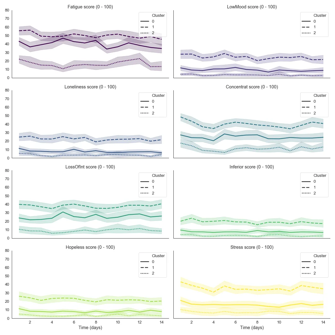
Figure 11. Average of each questionnaire variable per day and cluster.
As we can see in the Figure 11 (variable LowMood), the variability of the data over time is minimal and, in fact, although the result of the statistical test is statistically significant (f(13,26) = 2.261, p = 0.018), the effect size is practically negligible (η2 = 0.02).
Therefore, the repeated measures ANOVA statistical model has informed us that, despite having a dataset with detailed observations over time, symptom scores changed little over the observed period.
4. Regression Analysis
The first step we took to fit the linear regressions was to calculate the means of all the measurements by participant and variable. This allowed us to “remove” the temporal “repeated measures” aspect of the study.
Next, we build scatter plots between all the study variables, and we calculate the Pearson linear correlation coefficients (r) for combinations of variables, to identify strong associations and possible multicollinearity.r > 90%).
We observed that some variables were highly linearly correlated, as can be seen in the graph below:
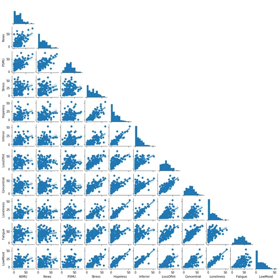
Figure 12. Matrix diagram of the scatter plots of the 11 study variables.
To fit an initial model, we had to define a variable “response” or “Y". We choose "LowMood”, because it is in principle one of the most important variables of the study.
In the heat map of Pearson linear correlations, multicollinearity is observed between “Loneliness and Hopeless", and "Inferior and Hopeless”, so we decided not to use “Hopeless”.
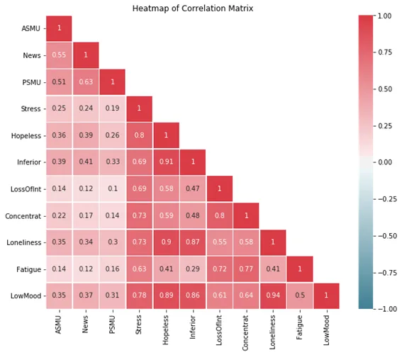
Figure 13. Pearson correlation coefficients heat map
of the 11 variables of the study.
For adjustment of the Regression Model, we use the method “backward”: from the model saturated with all the available independent variables, the method eliminated, one by one, said variables whose p-value > alpha, being alpha = probability of “type 1 error”.
We created a function called “calculateRegression”, which uses 80% of the data for adjustments, and reserves 20% of the data for testing.
Additionally, the function calculates the “RootMeanSquareError” (RMSE) and the “Coefficient of Determination” (R2) for each fitted model.
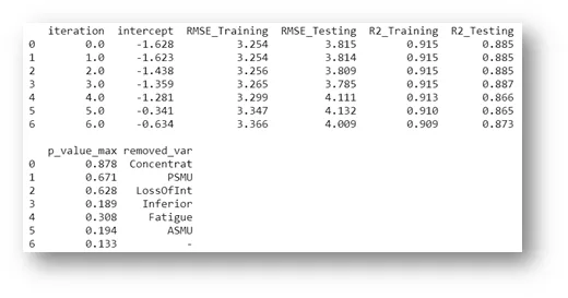
Figure 14. Output of the backward elimination procedure for removing variables with little explanatory power.
The Final Model adjusted involves 3 variables, being “News” one of them.
LowMood = -0,85 + 0,78 Loneliness + 0,18 Stress + 0,04 News
It is important to highlight that the coefficient of determination (R2) of the adjusted model is “high” (93.1%).
To examine some model assumptions, we performed a “residual analysis”, also collected in a function called “residualAnalysis”. This function performs the “normality test” (Kolmogorov-Smirnov) of the standardized residuals and prints 3 graphs: Scatter Plot between “Prediction” and “Standardized Residuals”, Histogram of the Standardized Residuals, and “Normal Q-Q Plot” of the Standardized Residuals.
The team considered the residual analysis satisfactory. This supports some checks on model fit, but does not constitute definitive or clinical validation.
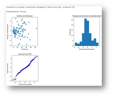
Figure 15. Output of the function “residualAnalysis”.
It is important to note that the weight of “News” (0.04) is much lower than the weights of “Loneliness” (0.78) and “Stress” (0.18), and that, if we had defined a “alpha” threshold, “News” would not be maintained in the final model.
To compare a different outcome, we constructed a “exploratory symptom index", to be used as a response variable of a second model. The idea was to compare the 2 models, in order to corroborate the previous conclusions.
The index, which we call “DeprRate", was calculated as the simple average between "LowMood”, “LostOfInt” and “Hopeless”. This variable was constructed for the analysis; it is not a validated clinical scale.
We follow the same steps outlined above. The final model now contains 5 variables and does not involve any variable related to the use of Social Networks.
DeprRate = -0,025 + 0,31 Loneliness + 0,25 Inferior + 0,19 Concentrat + 0,15 Stress + 0,06 Fatigue
The second model obtained an R² of 90.8%, with a residual analysis the team considered satisfactory. These are results from fitting these data, without clinical or external validation.
It is interesting to note that “Loneliness” again appears as the variable with the greatest weight for “DeprRate", and that "Stress” continues in this second model, with a similar weight.
Note: the two functions discussed above are defined in regresion_functions.py. The file also includes other functions used in this analysis, such as:
- printMatrixDiagram: function that generates scatter plots (2 to 2), involving all the study indicators. Useful to see graphically, at a single glance, the indicators that are most correlated with each other.
- printPearsonCorrelations- Generates a heat map of Pearson correlations between all indicators in the study. Useful to see, at a single glance, the indicators that are most correlated with each other and if there is multicollinearity.
- eliminateOutliers: eliminates the standardized residuals considered “high” (less than -3 and greater than +3), in order to subsequently make new adjustments without this data, which often distorts the results. The function prints the deleted data, allowing control of what is being deleted.
- repeatRegression: refits the final linear regression model fitted in “calculateRegression”, now for the data free of “outliers". Also, recalculate the "RootMeanSquareError” (RMSE) and the “Coefficient of Determination” (R2).
Final Conclusions
In relation to Cluster Analysis, it is observed that the 3 clusters formed are different as far as “depression symptoms” are concerned, the Cluster 1 the one that contains the highest means in relation to the 8 symptoms of the study. However, the same does not happen with the Social Networks variables, since the histograms overlapped by cluster they do not show great differences for the variables PSMU, News and ASMU.
On the other hand, the Repeated Measures ANOVA found a statistically significant but small time effect (η² = 0.02) over the 14 days. The original conclusion of “no significant differences” did not match the p-value of 0.018 reported above.
The Regression Models Adjusted results indicate that the use of Social Networks has a much lower weight than the other variables used in the study to explain a possible depression.
The Loneliness, the feeling of inferiority, the loss of Concentration and the stress they have a noticeably higher weight for this data set.
This finding coincides with the results of the Cluster Analysis presented previously.
All conclusions presented here refer solely and exclusively to the data set used in this project. To make more conclusive inferences, the study would have to be expanded using a larger sample, among other things.
Future Steps
In this dataset, social media use variables contributed less to modelling symptom scores than loneliness, feelings of inferiority, concentration, stress and fatigue. These associations cannot diagnose depression or establish what causes it.
As a possible research direction, the team proposed exploring natural language processing. Any tool used with people would require independent evaluation, consent and data protection; these results do not validate depression detection from social media posts.
Acknowledgments
We thank the mentors and organizers of Saturdays.AI Donostia, especially to Beñat Galdós and Joxemari Gallastegi, for their professionalism, dedication and enthusiasm.
Project presentation: DemoDay
Repository
In the following repository you will find the code used to develop this application: https://github.com/SaturdaysAI/Projects/tree/master/Donostia/Donostia2020/AISaturdays-depresion-rrss
More artificial intelligence!
Saturdays.AI makes AI more accessible through shared learning and projects with a social purpose. Our motto is AI4ALL IS AI4GOOD.
A story from the Saturdays.AI community. Originally published on March 16, 2022.
← More community stories