Take it to heart: Detection of malignant breast cancer tumors with Artificial Intelligence

Editorial note: this article documents an educational project and its results on the data used. It does not establish clinical validation or authorisation to diagnose or treat patients. Proposed healthcare applications are retained as the team’s goals, not demonstrated capabilities.

https://www.nationalbreastcancer.org/breast-cancer-facts

La Paz. Machine Learning. Second edition. 2020

Introduction

Breast cancer is the leading cause of death from malignant tumors in women worldwide. At least in 2019, around 688 thousand died due to this condition, which gives us a mortality rate for women over 20 years of age of 24.7 per 100 thousand.

Motivation

There is a breast cancer mortality gap between countries by income level, with 70% (483,000) of deaths occurring in low- and middle-income countries. Why? It happens that in low- and middle-income countries, there is a lack of access to diagnosis and treatment services for this disease.

Mortality and incidence rate

1. North America 22%
2. Latin America and the Caribbean 38%
3. Sub-Saharan Africa 65%

Between 50 and 63% of breast cancer deaths worldwide are preventable with early detection and appropriate treatment. Between 66 and 74% of these preventable deaths occur in developing countries. Likewise, breast cancer, detected early and with adequate treatment, can be cured. And if not, it can increase the quality of life of patients for at least 5 years (in North America).

Our social project arises from this problem. We know that the situation is very unfavorable for women, so we can contribute to generating a machine learning model that can help predict this type of tumors with which, in the future, many women could access a cheap and decent detection method, thus increasing their quality of life when faced with this genetic disease.

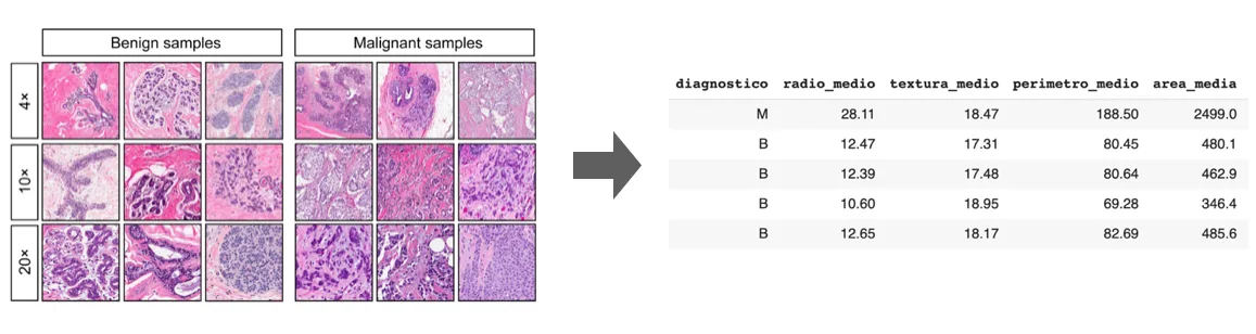
Breast cancer detection using the Wisconsin Diagnostics dataset

Objective

Explore different ML algorithms (Machine Learning) supervised and unsupervised using the Wisconsin diagnostic dataset (explained later), to compare them and verify which one provides us with the best breast cancer detection model, as well as review which variables provide the most information about detection.

The objective would be to propose a generalization of the database that could be implemented in any country to which this diagnosis is carried out.

Project

We worked on a comparison of certain supervised and unsupervised models to determine the accuracy of each one and subsequently use it for prediction.

Dataset

The data that we are going to use for this first exercise are those provided in the Wisconsin diagnostic dataset which contains variables about the shape of the tumor (in terms of cell nuclei) and its diagnosis, as shown below:

1. id: tag by observation.
2. diagnosis: binary variable that classifies the tumor. (M=malignant, B=benign)
3. radius: average of the distances from the center to the perimeter.
4. texture: standard deviation of the gradient values of the images.
5. perimeter: measurement of the contour of the cell nucleus.
6. area: measurement of the area of the cell nucleus.
7. smoothness: local variation of radius lengths
8. compactness: measurement calculated by ((perimeter²/area) -1)
9. concavity: severity of the concave portions of the contour
10. concavity points: number of concave portions of the contour
11. symmetry: similarity between parts with respect to axes.
12. fractal dimension: comparative index on the detail of an observed pattern of cells.

From variables 3–12 we associate the metrics: mean, standard error, extreme error.

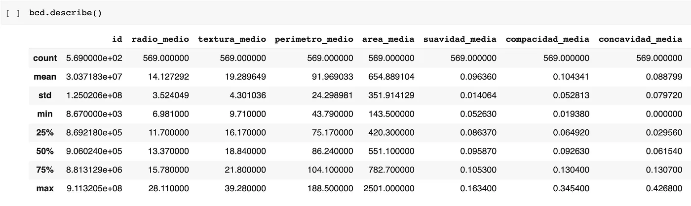
Description of the dataset with its metrics

Exploratory analysis

After having reviewed the variables of the dataset, we proceed to evaluate the distribution of the feature diagnosis to know the balance of the data, this has an impact when training the models, because as we can see in the following graph it has a greater amount of data associated with the diagnosis of benign tumors.

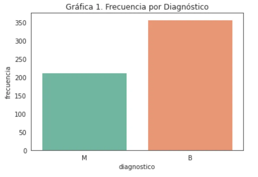
Diagnostic variable

Later we will proceed to see the correlation maps between variables to identify if any preprocessing needs to be done before training the models.

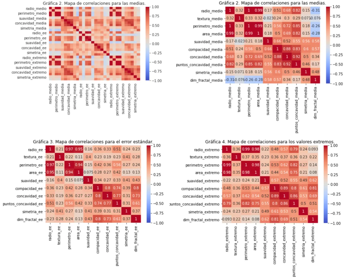
Correlation map with metrics

The previous graphs illustrate that in general the three maps show similar correlations, the averages show a more intense correlation than the extreme values and in turn, the extreme values show a clearer correlation than the standard error, however in the three maps the trend between variables is maintained.

We will highlight the most obvious correlations:

1. radio with perimeter/area/points of concavity: It is due to the way these variables are calculated, they depend directly on the radius.
2. perimeter with area/concavity/points of concavity: these correlations have to do with what was mentioned in 1.
3. softness with compactness
4. compactness with concavity/points of concavity/symmetry

Then, more specific correlation maps were made that include the three metrics of the variables with the most prominent relationships mentioned above.

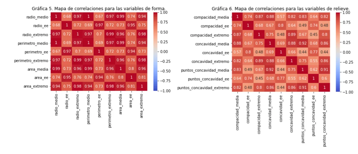
Correlation maps with the three metrics

The following graph has a particularity, it is observed that for the area metrics the extremes are highly correlated with the mean. And the standard error is the least correlated metric with respect to the other two.

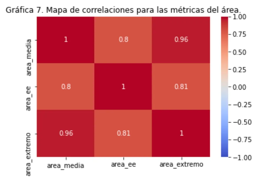
Area correlation map

Finally, we will show the distributions and scatter diagrams for the average by type of diagnosis, which gives us an indicator of how the densities behave that can be included in the following groups:

1. There is a almost total separation between densities: they share neither form nor support.
2. There is a regular separation between densities: share form or support.
3. There is a minimum separation between densities: share shape and support except for slight variations.

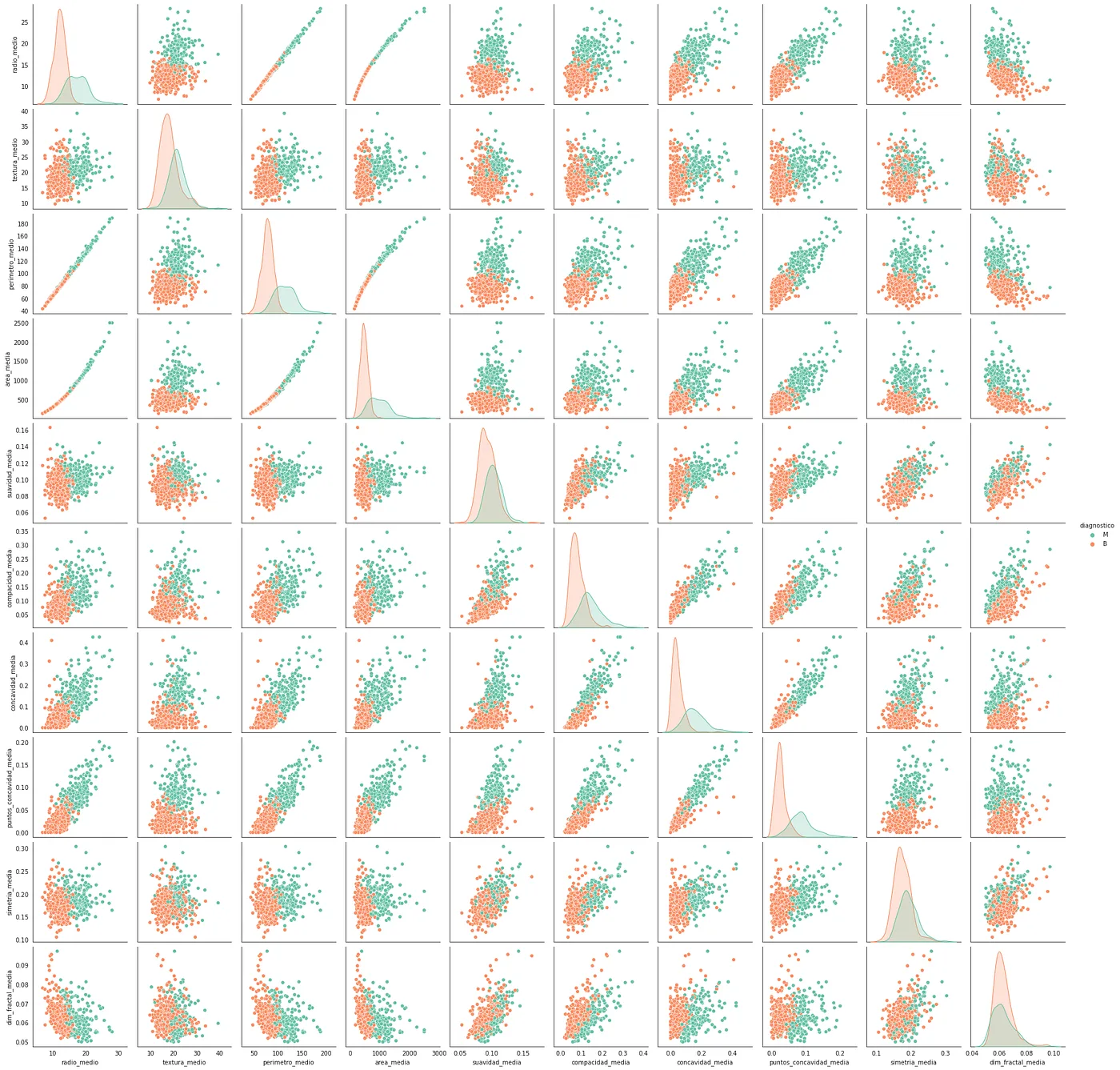
Distributions about the mean using the variable diagnosis

Unsupervised algorithms

PCA

We propose this analysis because the structure of our database has a high dimension (30 variables) Therefore, this unsupervised analysis technique will help us reduce the number of components (variables) in our database, projecting the original variables to a subset of them.

The final set of essential variables after this analysis will eliminate those that are possibly correlated. We now have a a priori approximation which will be defined with this analysis, given that we want to form two clusters due to the binary form of our objective variable. diagnosis.

The following table shows the percentage of variance accumulated by each of the main components. In principle, we consider 10 main components, as seen in the table, the first and second components explain the 44.27% and 18.97% of the variance respectively, which implies that the first two components explain the 63.24% of the variance.

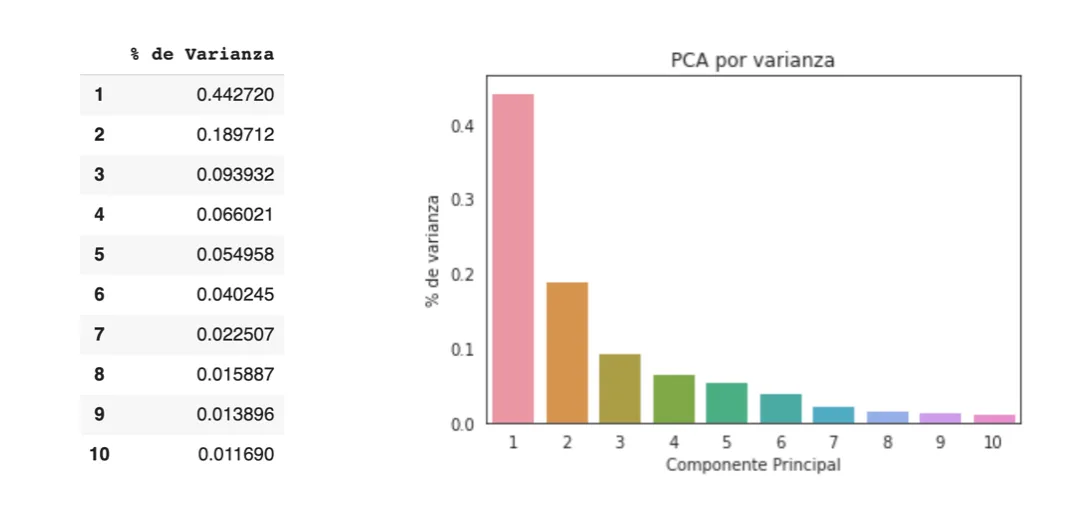
PCA with n_components = 10

So we will repeat the procedure but for now only remove 2 components, since they obtain more than 60% of the total variance.

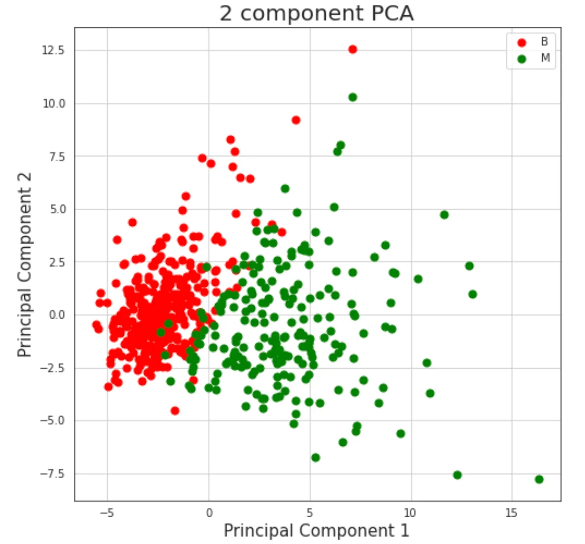
2-cluster distribution for the variable diagnosis

Now we are going to try it with n=3 and we can observe the same behavior as with two dimensions. In conclusion there is a clear grouping with respect to type of diagnosis, could even be separated linearly (with a straight line in the two-dimensional case and with a plane in the three-dimensional case) except for some observations that are completely disseminated.

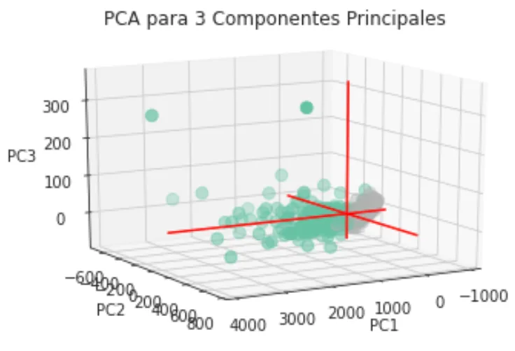
PCA n_components = 3

K-Means

For this ML algorithm, we used the dataset without reduction, and we trained the model to maximize the separation of the clusters given the characteristics we have (28 variables, removing the label).

In this case, a silhouette-type visualization can help a lot to explain the results. The Silhouetter Score fue de 0.697 That is, how well separated the clusters are, remembering that 0 means that there is overlapping and 1 means that they are perfectly delimited.

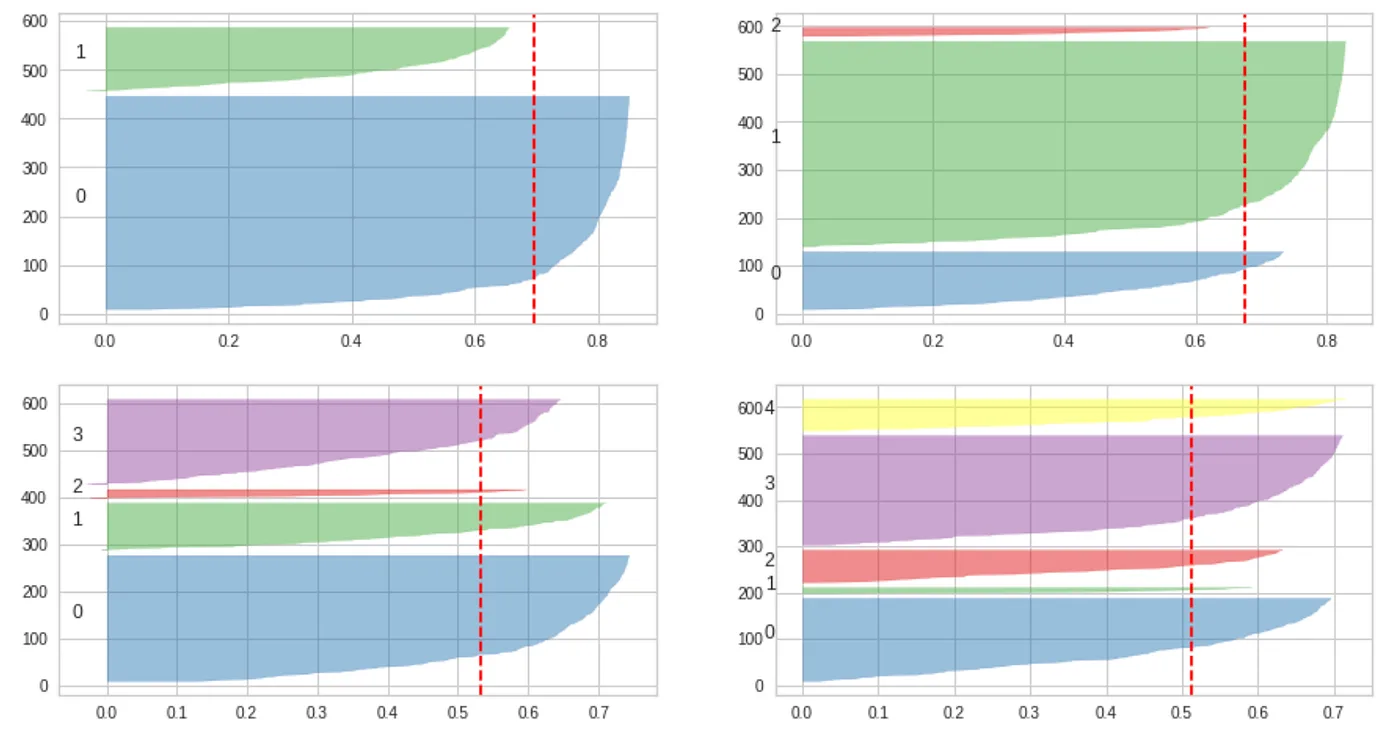
Silhouette visualization for the 2 main clusters of the diagnostic variable

To test this model we decided to generate random data with the variables selected from the dataframe and these were the results:

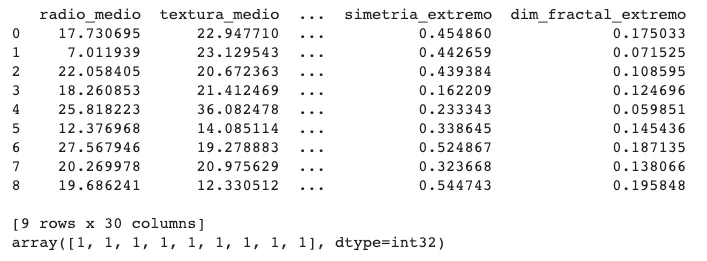
The model is capable of classifying whether they are 1 (Benign) and 0 (Malignant) depending on the incoming values that were generated randomly. This later with real data, could detect breast tumors with up to a probability of 69%, which is undesirable. Later with supervised algorithms we will be able to increase this percentage.

Supervised Algorithms

Logistic Regression

Our project falls into the binary classification category, because we have a variable diagnosis which only shows us if it is benign or malignant. Therefore, this model benefits us by giving us a first approximation to solving the problem. In the first instance, we apply the logistic regression algorithm to the data in its 30 dimensions and to clearly see how this classifier is working, we will use a confusion matrix as shown below.

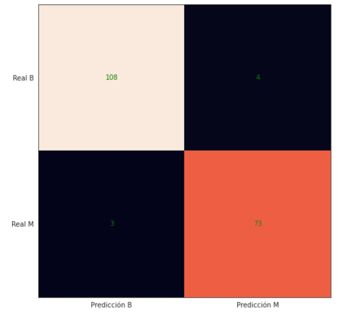
Confusion matrix on false positives, false negatives, true negatives and true positives

Given the previous prediction we can include the model accuracy calculated with the sklearn metric accuracy_score was from 0.962765. Result that is much better than our previous unsupervised model (KMeans).

A more specific diagnosis is the prediction probability per observation, that is, how likely it is that that observation will be classified as Benign or Malignant. So let's see their performance by cross-validation. Cross-Validation Accuracy Scores [0.94871795 0.92105263 0.94736842 0.92105263 0.97368421 0.97368421 0.97368421 0.94736842 0.92105263 0.94736842].

From the above we conclude that on average we have a precision of 94.6%However, it is necessary to review the structure of the model and its assumptions.

Logistic Regression step by step

After the first approximation of the model, it is time to review whether certain assumptions required for the development of logistic regression are met. We will list some of these assumptions below.

1. The target variable must be binary. In our case diagnosis is 'M' or 'B'.
2. The result of the variable of interest associated with “success” must be 1.
3. Only significant variables should be included.
4. The variables must be independent of each other, to avoid multicollinearity problem.
5. There must be a “sufficient” sample size

We will proceed to the construction of the linear regression taking care of these assumptions.

At first we detected that our sample was not balanced in the number of malignant (~37%) and benign (~62%) observations, for which the library was used SMOTE because it performs a random generation of the missing observations based on KNN.

Balanced the observations to have the same number of B and M observations

Note: We only oversample on the training data set, since the information that is in the test data will not be incorporated into the training model.

For “Only significant variables should be included”, it is necessary to identify the variables that have the best performance, so that smaller and more representative variables or characteristics can finally be included. These were the variables chosen:

“mean_radius,”,”mean_texture,”,”mean_perimeter,”,”mean_area,”,”mean_smoothness,”,”mean_compactness,”,”mean_concavity,”,”mean_concavity points,”,”mean_symmetry,”,”mean_fractal_dim,”,”ee_radius,”,”ee_texture,”,”ee_perimeter,”,”ee_area,”,”ee_smoothness,”,”ee_compactness,”,”conc avity_ee”,”points_concavity_ee”,”symmetry_ee”,”dim_fractal_ee”,”radius_extrem”,”texture_extrem”,”perimeter_extrem”,”area_extrem or”,”smoothness_extreme,”,”compactness_extreme,”,”concavity_extreme,”,”points_concavity_extreme,”,”symmetry_extreme,”,”dim_fractal_extreme”

Now we will implement the model with the new variables selected and the balanced data:

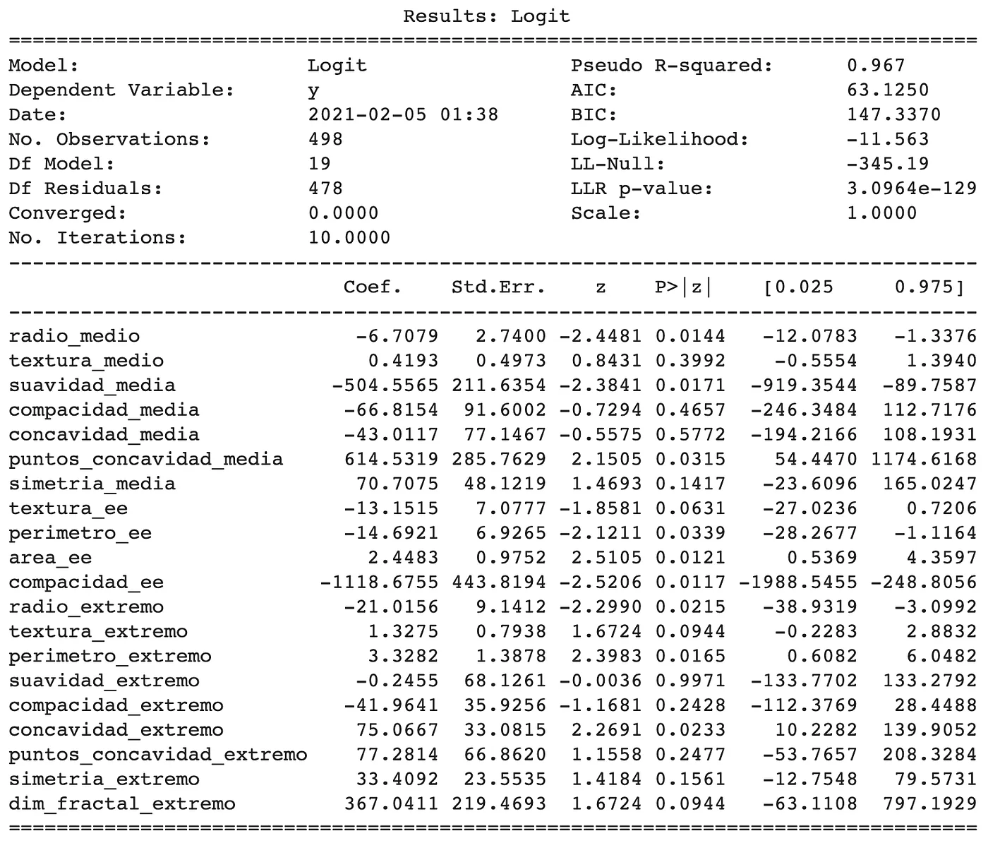
By manually checking the p value of each of the variables, We remove those such that the p value exceeds .05, which is our confidence level. Now we are going to review the assumption of independence, we will again review the correlations with the final variables of our model.

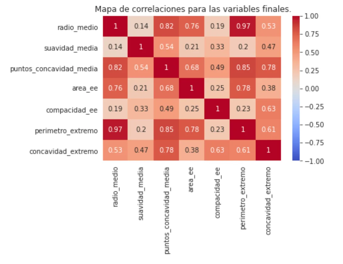
Correlations for final variables

The correlation map above suggests a high correlation for medium_radius and extreme_perimeter so we will remove one of the two based on the rating obtained in the model's performance.

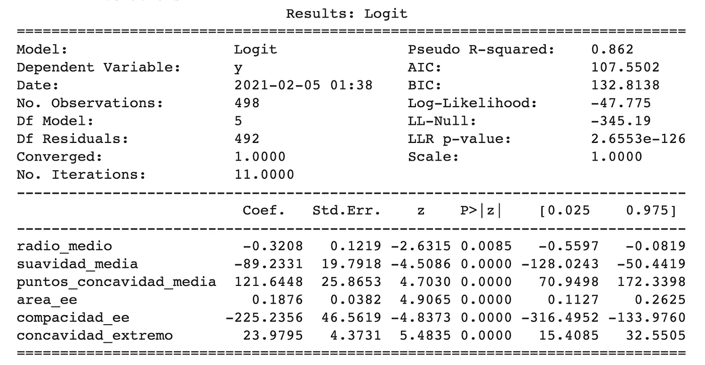
Logit on the model and see the best middle_radius vs end_perimeter score

Now the selected variables show a generally low correlation, which contributes to the independence hypothesis. Now we will rate the performance of our model again. First we will obtain the new confusion matrix and then the precision.

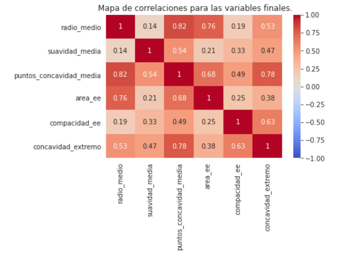
There are no longer dependent variables or variables with high correlations

Now our precision is 0.918. This is what the confusion matrix looks like:

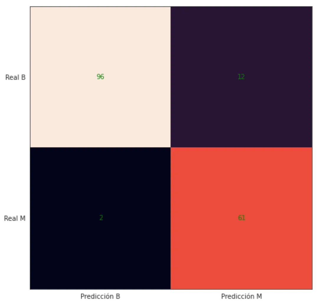
confusion matrix

Finally, let's check with a ROC Curve which is a tool used in binary classification models, the way to interpret this graph is that an accurate classifier must be as far away from the identity line (except at the extremes).

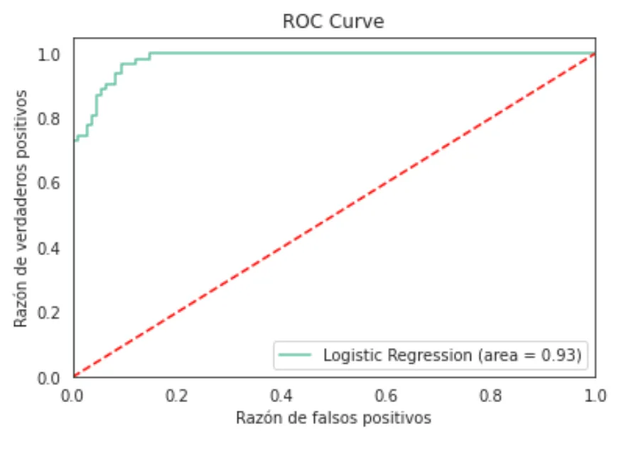
ROC Curve to verify model accuracy

After this processing, we can conclude that we have an accuracy of 92% on average which is lower than that proposed in the first logistic regression model, the advantage of this last model is the dimension reduction from 30 variables to 6 in addition to being more in line with the assumptions of the Logistic Regression model, this can have implications in terms of generalization (working in other databases) and computational cost (less processing time).

SVM

This algorithm aims to classify different classes of observations based on distances to hyperplanes; it is preferred due to its level of precision and low computational cost. Furthermore, another advantage of this algorithm is that it works well for large dimensions, that is, for a large number of explanatory variables.

After this implementation we obtained a precision of 92.98% However, there are certain observations that are important to highlight about this algorithm.

• This algorithm is not very precise when there is no clear separation between the classes of variables. In our case, it can be seen in the PCA visualization that there are observations that are mixed between classes.
• This algorithm optimizes distances, meaning that there is no statistical basis for the classification, it does not consider the distribution of the data.

KNN

We will now implement the KNN algorithm, which is a non-parametric algorithm frequently used as a classification or regression model.

We will first plot the number of clusters that maximizes the function.

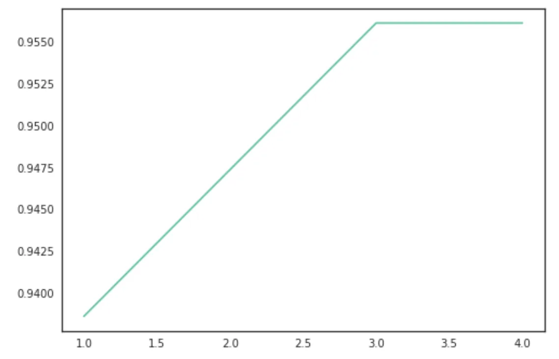
Cluster maximization

We obtained a precision of 96.27% which is greater than the precision obtained in the previous models, however, certain observations must be made about this model:

• This model does not perform well when there are a large number of variables. This implies that for a fixed level of precision, as the number of explanatory variables grows, the number of observations must grow exponentially.
• It has little generalization power, that is, it has overfitting problems.
• The above points imply that there is a large computational cost to run this algorithm.

And last but not least…

Random Forest

As we expected, this model has an accuracy of 97.36% which is the highest compared to the other models, some comments about this model are:

• This model is fundamentally predictive, not explanatory, it does not have a clear sense of information processing.
• For complex problems the computational cost can grow too high.

Conclusions

After testing the previous models we noticed that each of the implementations has advantages and disadvantages, there are also models that complement each other as we see in the case of PCA, logistic regression and SVM, where an unsupervised learning model can trace the possibilities of classification and dimension reduction, subsequently implement a supervised learning model for the prediction of the dependent variable.

Each problem has a particular context that must be considered for the proposal of specific models, the quantity and type of explanatory variables configure the reference framework for the implementation of models.

In the particular case of our problem, the prediction objective of the dependent variable diagnosis It can be approached in general from two perspectives:

• On the one hand, we have the goal of predicting with the greatest precision whether the diagnosis for the patient is favorable or unfortunately unfavorable, according to the metrics obtained if we follow this single goal, the model of Logistic Regression It gives us a higher precision than the others which translates into a minimum error when classifying, however its generalization to other databases related to this problem is questionable.
• On the other hand, we have the goal of generalizing this model to other databases, so in this sense we lean towards the Logistic Regression model step by step, since in addition to the fact that it adheres better to the specific assumptions of the model, it reduces the dimension of the problem from 30 explanatory variables to 6 variables, the latter has a positive impact in terms of computational processing and data storage/collection.

It is true that for the generalization objective we lose percentage points of precision (given that step-by-step Logistic Regression has a precision of 92% on average) but the advantage of generalizing this model is a priority specifically given the mortality figures that are currently associated with breast cancer.

Extending this model to databases generated by other countries, especially those with lower income and worse public health coverage, translates into shorter waiting times for diagnosis, lower costs of procedures, and timely treatment for patients.

Another advantage in practical terms that follows the same axis is that the relevant variables included in the final model are 6, which represents an 80% decrease in the dimension of the problem. For countries with a lower budget for research and health, it will be cheaper to create databases with only 6 metrics per observation, and the storage and subsequent processing of information will also be easier and more timely..

References

The data presented in the introduction was obtained from the following articles:

• http://tomateloapecho.org.mx/Pdfs/Numeralias/2020/FS%20CAMA%20ESP%20(09-20).pdf
• http://tomateloapecho.org.mx/Pdfs/Numeralias/2019/Numeralia%20MEX-MUNDO%202019.pdf
• http://tomateloapecho.org.mx/Pdfs/Numeralias/2016/Cancer%20de%20mama%20y%20mujeres%20jovenes%20en%20America%20Latina%20y%20el%20Caribe.pdf
• https://www.aprendemachinelearning.com/k-means-en-python-paso-a-paso/
• https://rstudio-pubs-static.s3.amazonaws.com/344010_1f4d6691092d4544bfbddb092e7223d2.html

Members

• María José Sedano Castañeda
• Dante Fernando Bazaldua Huerta
• Carlos Alberto Gomez Vazquez

Project presentation: DemoDay

Open video or resource

Repository

In the following repository you will find the code used to develop this application: https://github.com/SaturdaysAI/Projects/tree/master/Lapaz/2021.ML2/Equipo%204

More artificial intelligence!

The mission of Saturdays.ai is to make artificial intelligence more accessible (#ai4all) through intensive courses and programs where projects for good are carried out (#ai4good).

Explore our AI master’s programme at https://saturdays.ai/master-ia-online/

If you want to learn more about artificial intelligence join our community at community.saturdays.ai or visit us on our website www.saturdays.ai Join us!