Prediction of desertification zones using AI.

Zaragoza. First Edition. 2022

Desertification is caused by land degradation which occurs in dry areas: arid, semi-arid and dry subhumid. Human activity and climate variations are among the causes of this soil degradation, which impacts ecosystems and resources and ways of life of the inhabitants of the affected areas. These dry areas are those with an aridity index (AI=P/ETP) less than 0.65.

Spain is one of the territories that suffers from this problem. In Aragon, 75% of the territory is at risk of desertification. Climate change and increasing temperatures threaten the semi-arid lands that predominate in the Ebro Valley, from the city of Huesca to the south. Identifying these areas in time will be of great help to support the taking of actions that will mitigate the impact that desertification brings on food security as well as reducing the loss of natural habitats and biodiversity, all of this, aligned with the United Nations Sustainable Development Goals.

Focus on Sustainable Development Goals 13 and 15. Source: https://sdgs.un.org/goals

To identify these areas, a process is proposed that manages the recognition through satellite images of the desertification areas in Aragon and allows an approach to be made to predict possible future desert areas with the aim of applying more efficient policies regarding the reforestation of the affected areas, and new crop treatments. With support from the initiative Saturdays.AI Zaragoza, whose objective is to bring AI closer to all citizens and apply it to social problems, we want to provide a solution or an approach to resolve this scenario that we have considered as a work team.

It is then when we ask ourselves the following concerns: How is it possible to calculate whether or not there is desertification in a given area? What images can work for this purpose? How can AI support us to predict these values? Throughout this article we will try to solve these questions.

Satellite Images

Remote sensing tools make it possible to visualize and calculate changes that occur on the Earth's surface, those that interest us, those that correspond to passive remote sensing (Definition of Remote Sensing), in our specific case, they capture the solar radiation reflected by the surface. It is well known that living organisms reflect and absorb solar radiation differently than inert objects such as streets or buildings. Taking advantage of this principle, satellites generate images that contain these differences in the form of Digital Levels and bands, which are translated into numerical units that correspond to the wavelength values of the different sections of the electromagnetic spectrum (Electromagnetic spectrum and remote sensing). In short, they measure the radiation reflected by objects such as buildings or highways or living entities such as forests or vegetation in general.

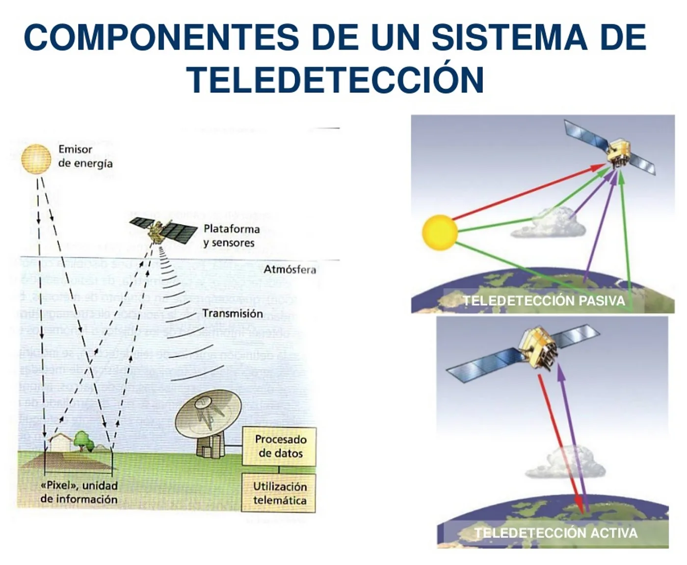
Main Components of a Remote Sensing System. Source: Remote sensing course https://static.uvq.edu.ar/mdm/teledeteccion/unidad-1.html

NDVI Vegetation Index

Changes in vegetation with the support of satellite images can be measured in different ways, one of them is by extracting vegetation indices, “Vegetation Indices are combinations of the spectral bands recorded by Remote Sensing satellites” (What is the NDVI Vegetation Index?) that allow identifying vegetation on the earth's surface. It is there, with the help of these indices, that the properties of the vegetation as such are highlighted and can be analyzed numerically.

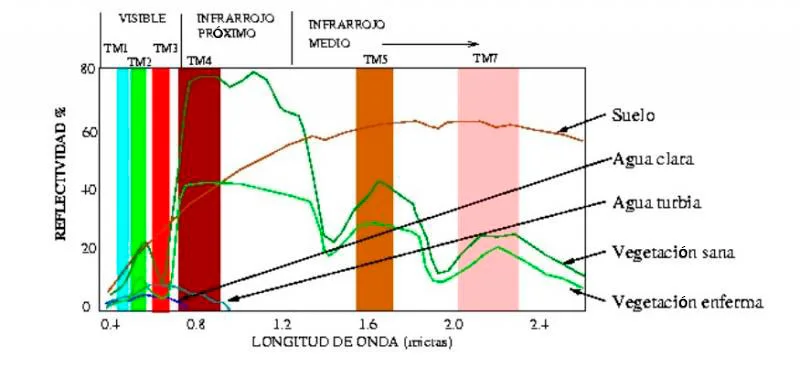
Interaction of the elements of the Earth's surface with radiation. Source: University of Murcia. Remote sensing notes. <https://www.um.es/geograf/sigmur/teledet/tema02.pdf>

The NDVI is the Normalized Differential Vegetation Index, NDVI for its acronym in English. This index is a calculated parameter that is based on the values captured by the satellite instrument where it identifies patterns of the electromagnetic spectrum that correspond to the reflectivity of vegetation covers. This index helps to easily distinguish vegetation in satellite images.

The patterns of the electromagnetic spectrum to identify vegetation show that vegetation absorbs the section of solar radiation that corresponds to red. At the same time, high values are reflected in the near infrared and we will be able to identify bright multispectral values in this band ( NDVI Spectral Values).

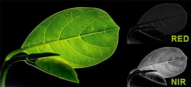
Representation of vegetation cover in RED and NIR. Source: NDVI calculation http://www.gisandbeers.com/calculo-del-indice-ndvi/

This way we can differentiate vegetal covers in different states. Our index can be obtained through the following relationship:

NDVI = (Near Infrared Band — Red Band) / (Near Infrared Band + Red Band)

Or what is the same, and in terms of nomenclature when we work with multispectral bands:

NDVI = (NIR — RED) / (NIR + RED)

Once the index has been calculated for each of the image pixels, the possible values range between -1 and 1.

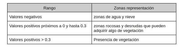
NDVI values for different areas. Source: own

The higher the value, the more lush the vegetation will be until it acquires values close to 1.

Manipulating the image

To better understand how we can use these values across bands and digital levels, it is important to identify the properties of an image in general and what these values look like at the computational level.

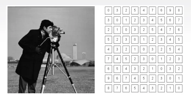
Right: how a human being sees an image. Left: how a computer processes it. Source: Material Satudays.AI, Zaragoza. Edition I. 2021–2022. Image Treatment.

The computer or computing methods structure the images into matrices with values (i,j) these values (i,j) numerically represent the value in computational terms of said coordinate on the original image (without digitizing). Each of these values is what is called a “pixel”.

For satellite images something similar happens, the only difference lies in the values for each pixel, in this case they represent in digital levels for reflectance values of solar radiation (electromagnetic spectrum) reflected by the terrestrial object on which the instrument (the satellite) is measuring.

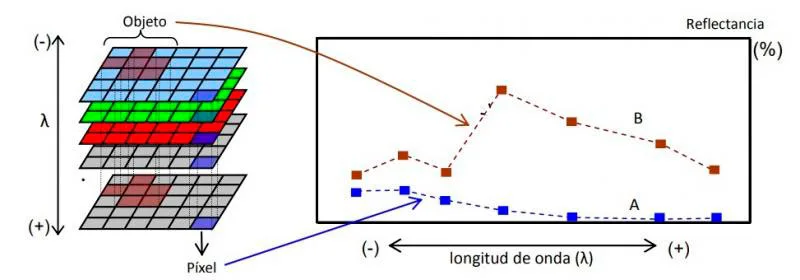
Spectral signatures in images. Source: Image 45. Use in multispectral images. https://static.uvq.edu.ar/mdm/teledeteccion/unidad-1.html

Data collection and preparation

Obtaining

Since an analysis will be carried out on changes in the Earth's surface, the satellite images that were chosen were from the Sentinel 2A instrument. To obtain data we use the Python library SentinelSat for downloading images in the area that interests us. It should be noted that the images have been taken with the following conditions: for a specific area detailed in a .json file, for the same tile (satellite image capture area) and orbit section to guarantee that the same study area is being taken for different moments in time.

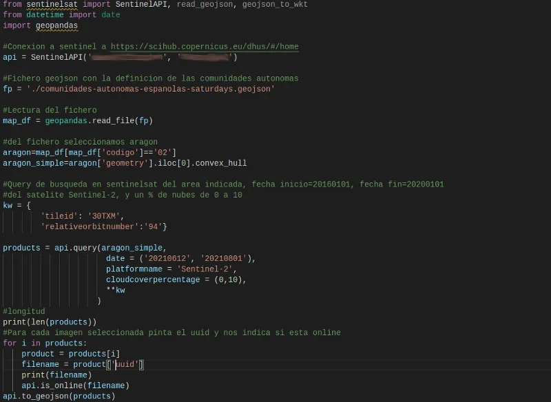
Code fragment for downloading sentinel images from the scihub.copernicus.eu site Source: Own

NOTE: To obtain and capture the data, Sentinel images have been downloaded with a maximum cloud percentage of 10%.

Once the script to download satellite images has been executed, a series of zip files are downloaded, each containing the following structure when decompressed:

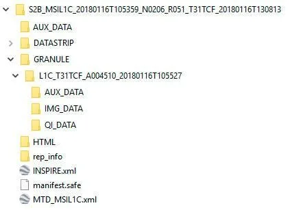
File structure downloaded from the scihub.copernicus.eu site Source: own

Each Sentinel image is given a consecutive image name with the following structure:

MS2_MSILLL_YYYYMMDD

Where:

• MS2: identifies the mission of Sentinel 2, being able to find S2A (for Sentinel 2A) or S2B (for Sentinel 2B)
• MSI: indicates the operating instrument (MultiSpectral instrument)
• LLL: indicates the level of processing of the product and can find levels L0, L1C, L1B or L2A
• YYYY: designates the UTC time point (year) in which the image was taken
• MM: designates the UTC time point (month) in which the image was taken
• D.D.: designates the UTC time point (day) in which the image was taken

Sentinel downloads for the project were:

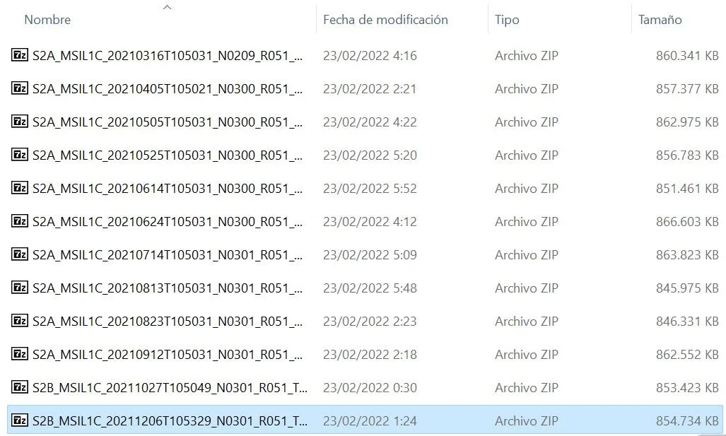
List of images. Source: Own

Preparation

Once the images are obtained, we will calculate the NDVI indices on them using a Python script.

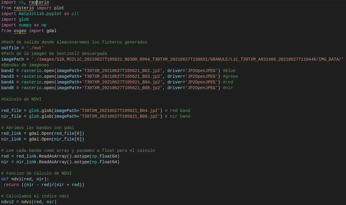
Code snippet for calculating NDVI for downloaded images

To understand the output of this script, the images with the calculated NDVI (new tif files), it must be taken into account that this image transformation gives us an image composed of a matrix of values where each value corresponds to a pixel (representation in the image) and this value ranges between -1 and 1. Remembering the Vegetation Index section, from 0.3 we understand that there is vegetation for that pixel (matrix value).

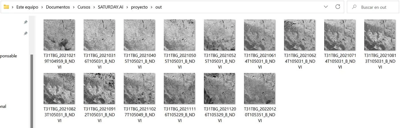
Screenshot of the NDVI images generated by the script. Source: Own

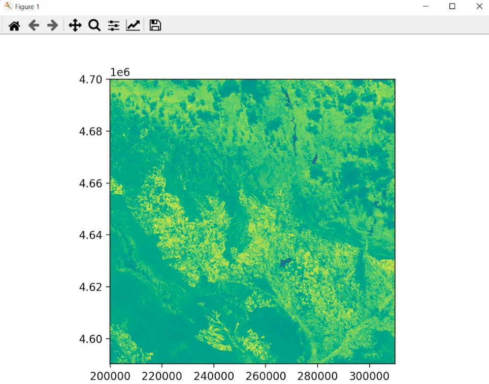
Detail of one of the NDVI images generated by the Python script. Source: Own

And the prediction of desertification values?

We are already at the point where, we have identified the area on which we will work, we have found the vegetation indices for these areas at different moments in time, now we will continue with the establishment of a relationship between the measured values and how they change over time (our continuous variable) to anticipate a set of new values.

We wish to build a model that describes the relationship between the study variables, with the aim, mainly, of predicting the values of one variable from the values of the other. we will choose Random Forest Regressor since we have a set of numerical values that we have considered as categories (each image with its specific matrix) and then we average the output of each decision tree using this algorithm (Definition of Random Forest regressor. Material Saturdays AI. Zaragoza. Edition I. 2021–2022. Session Regressors).

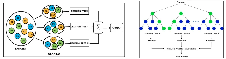
Brief summary of how Random Forest Regressor works

As this is a Supervised Machine Learning model, we will take the images with the calculated NDVI, only one area of ​​them for model learning and the next area of ​​the images for the future prediction of NDVI indices.

Evaluation

Training

For algorithm training, 5 images with calculated NDVI and one additional image as known output were taken. From each of the images, a subset of equal size has been chosen to add them to a vector in Python. The above is done due to the processing capacity of the available machines, the original images have dimensions of 10,000×10,000 pixels that cannot be processed quickly and efficiently with the resources available in the work group.

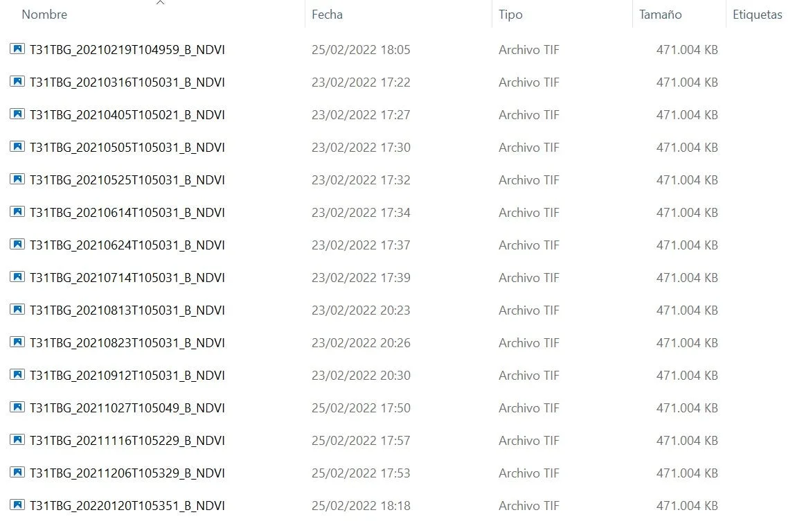
Images with NDVI calculated. Source: own.

Explanatory Note: Each calculated NDVI image has a size of approximately 470MB, so 6 of them gives us an estimated 2.8GB to process this dataset.

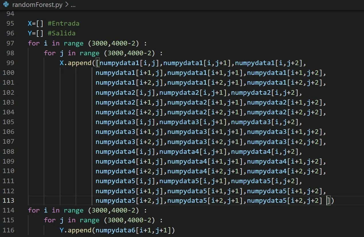
Code fragment for choosing the data subset for the training Random Forest. Source: own

With the help of the bookstore sklearn We establish a training set for the algorithm with which we can “teach” it how it can try to predict the following values and execute the next testing phase.

Test

To test the algorithm, the same 5 images were taken with the NDVI calculated but this time, the chosen subset corresponds to another portion of the image. In training we have chosen a section, for the test we choose a different section.

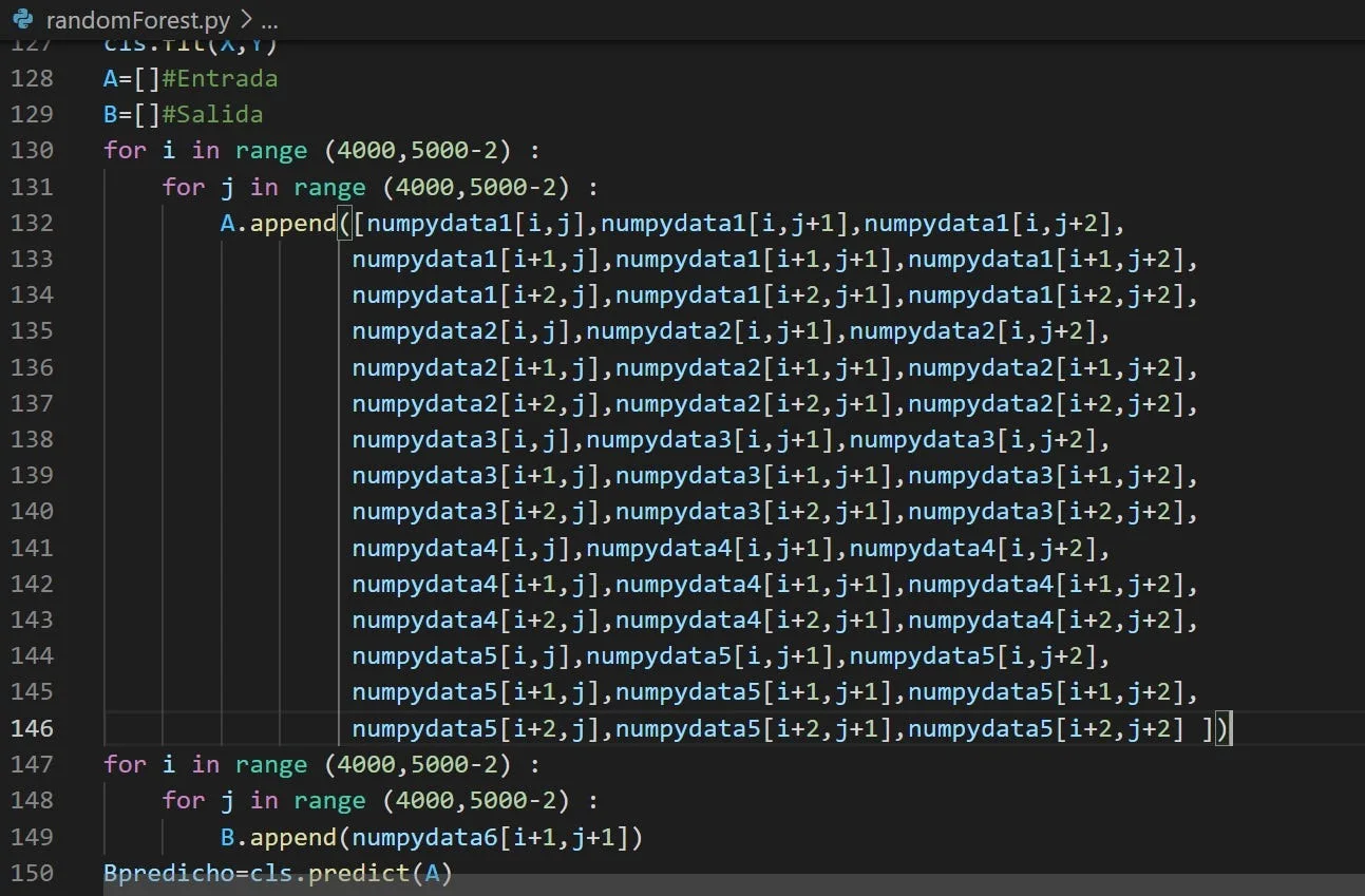
Code fragment for choosing test data for the algorithm. Source: Own

The margin of error for the predicted image is as follows:

Margin of error resulting from the prediction. Source: Own.

It is necessary to know if the algorithm is capable of correctly predicting an image. We will use an image that we already have to validate the effectiveness of the algorithm in predicting the result.

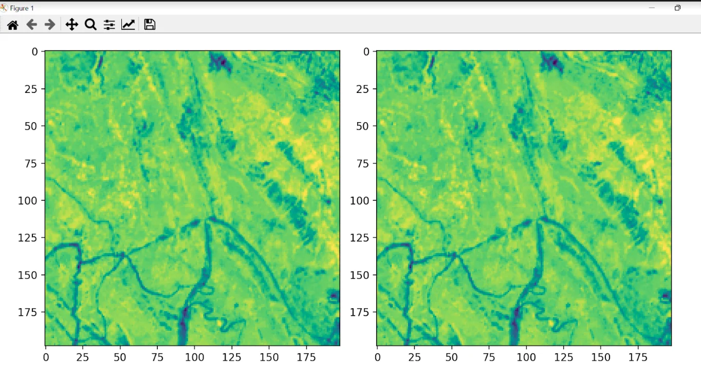
Right: Original image. Left: Predicted image. Source: Own.

Streamlit visualization

on the page desertIAragon The Streamlit application is deployed to view the changes in calculated NDVI

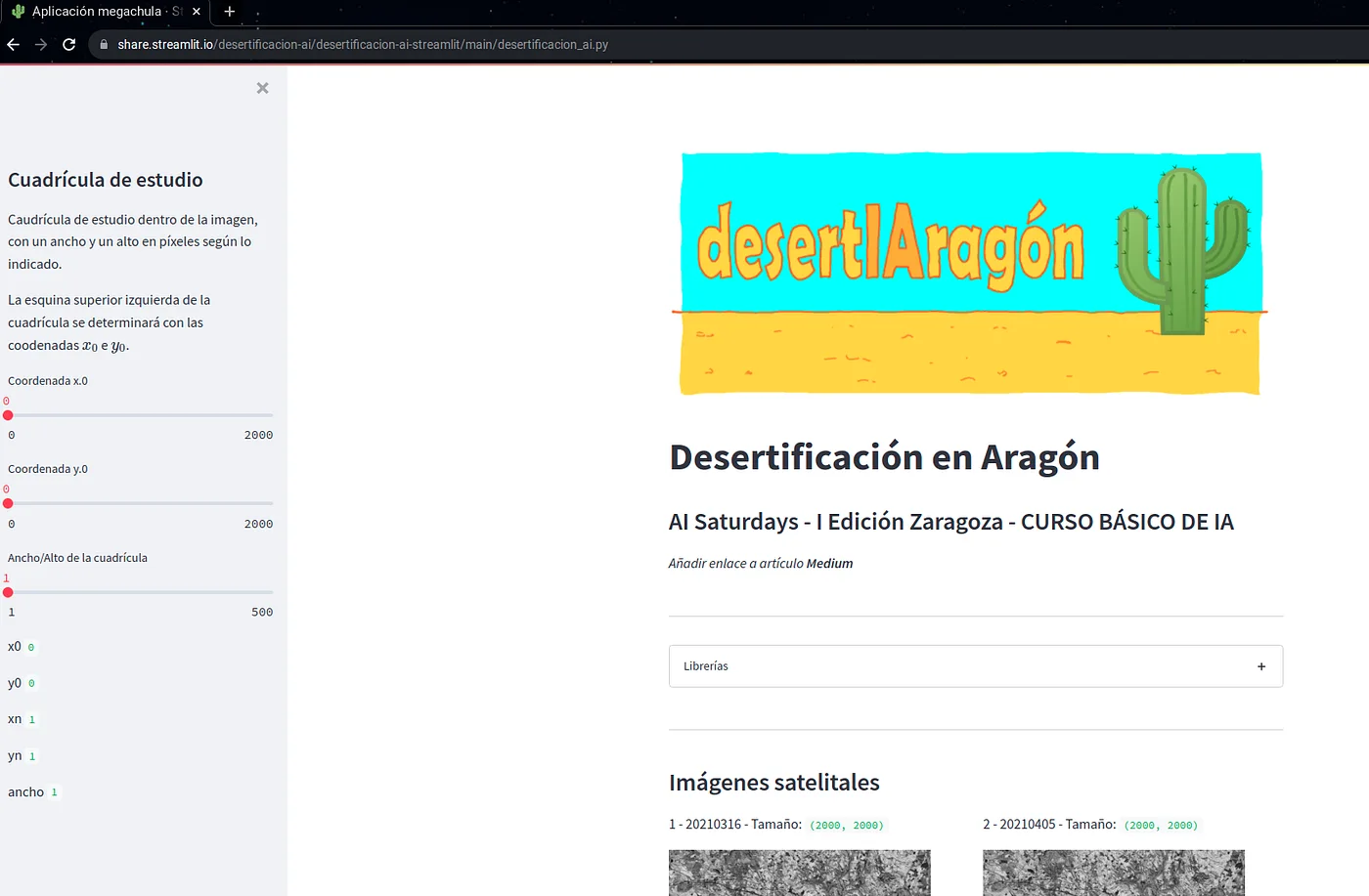
Screenshot of the Streamlit website to show calculated images. Source: Own

In the section Satellite Images, we find a 2000x2000 pixel subset of the images taken from the Sentinel website:

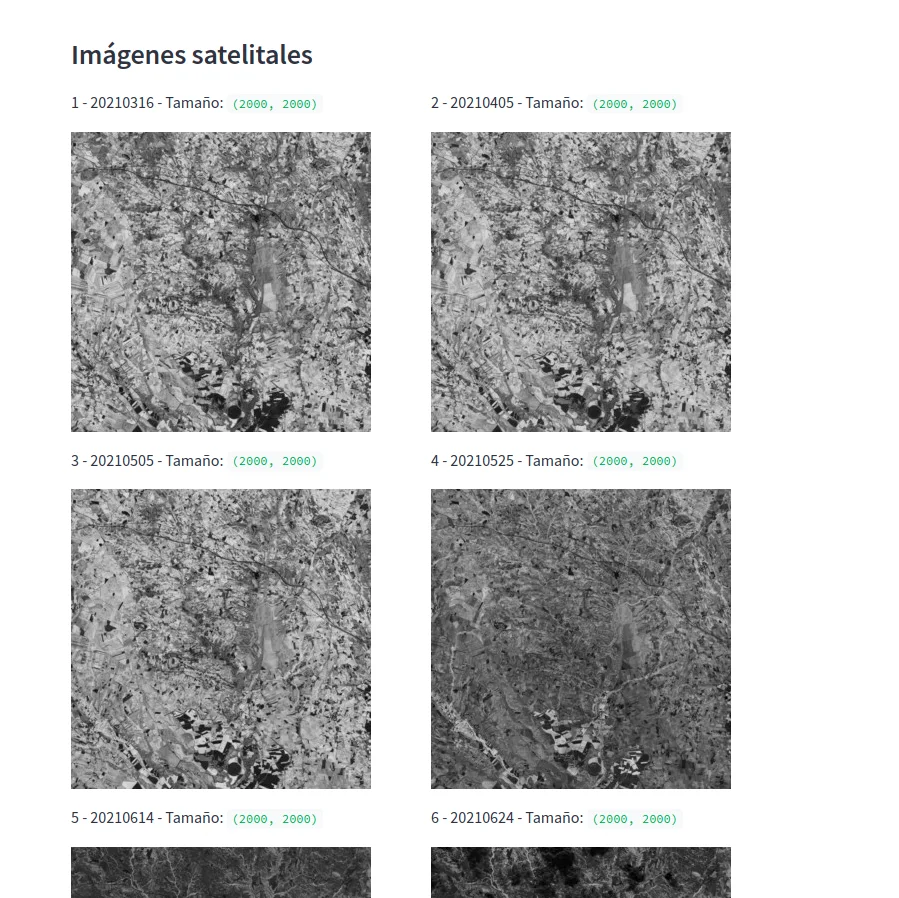
Satellite images of 2000 x 2000 px. Source: own

The study grids section allows us to choose the desired coordinate to display the changes in the calculated NDVI and its values. Choose the coordinate from the options available in the left panel:

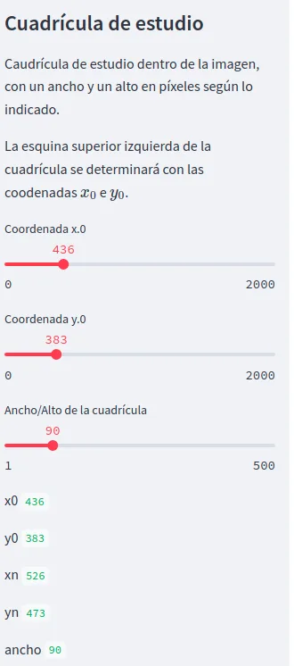
Choice of coordinate for the study grid. Source: own

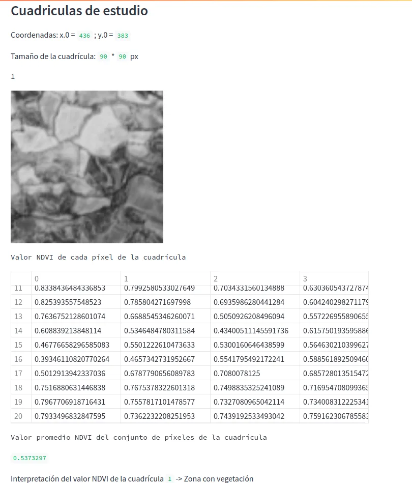
NDVI value calculated for image 1. Source: Own.

Prediction

The system is trained with an equal portion of each of images 1 to 5. This portion is a box of random coordinates and dimensions equal to the width/height of the grid indicated in the sideband (in Streamlit).

The reason for choosing a reduced box is the high computational cost of training the system. This cost may be around 5 minutes of processing for a fragment less than 250 pixels in size, on a computer with 8GB RAM and a processor: Intel Core I5 ​​2.67 Ghz.

In this way the application can show results in a relatively agile way. For the test, the images from grids 1 to 5 have been chosen with which the NDVI index has been obtained.

The prediction is made with grid 6. The original image is compared with the one predicted by the AI.

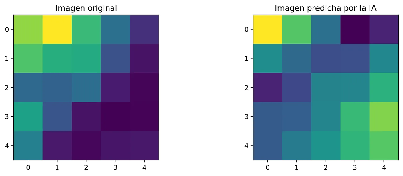
Comparison of fragment of the original image vs. AI predicted image

General image data:

Upper left corner coordinates: i_0_i_0​ * j_0_j_0​ = 0 * 0 px Upper right corner coordinates: i_n_in_​ * j_n_jn_​ = 5 * 5 px

Mean square error: 0.03719

Conclusions

• There is proprietary software such as ERDAS to facilitate the calculation of NDVI and regression algorithms to predict behaviors, however, aligned with the principles of Saturdays.AI: bringing AI closer to all citizens and applying it to social problems, we have opted for a solution based on open source tools available to the public.
• This project has the potential to explore as a next phase the data processing capacity for larger dimensional images, whether in spatial or temporal resolution, more efficiently in the cloud. Taking advantages such as parallel or distributed processing, it will be possible to add more inputs to the algorithm and more complex processing that cannot be supplied with current resources.
• Desertification over the evaluated areas can be predicted efficiently, with a fairly small margin of error for the first evaluation phase. At a numerical level it is possible to establish where vegetation has been lost over time and predict its future values ​​to take timely actions in these areas and thus avoid new areas of desertification.

Project members

Eva de Miguel Morales

Pedro Biel

Yineth Castiblanco Rojas

Project presentation: Demoday

See video

Repository

The code for this project can be found at GitHub

Additionally, the display code can be found at: GitHub Streamlit

More artificial intelligence!

The mission of Saturdays.ai is to make artificial intelligence more accessible (#ai4all) through intensive courses and programs where projects for good are carried out (#ai4good).

Explore our AI master’s programme at https://saturdays.ai/master-ia-online/

If you want to learn more about artificial intelligence join our community at community.saturdays.ai or visit us on our website www.saturdays.ai Join us!