AIreySalud: Air quality modeling with Artificial Intelligence

Latam online. First Edition. 2020

How to get ahead of the invisible enemy?

According to the World Health Organization, air pollution represents one of the greatest health risks, showing a direct relationship with the burden of morbidity derived from strokes, different lung cancers and chronic and even acute lung diseases, including asthma.

There are studies that confirm that aligning with the guidelines recommended by the WHO results in an impact of up to 22 more months in increasing life expectancy in the population (WHO, 2016).

air x-ray

In 2016, 91% of the population lived in places where laws were not respected. WHO Air Quality Guidelines. According to 2016 estimates, air pollution in cities and rural areas causes 4.2 million premature deaths. 91% of these premature deaths occur in countries of low and middle income, and the highest morbidity rates are recorded in the Southeast Asia and Western Pacific regions.

In low- and middle-income countries, exposure to pollutants in and around homes from the use of fuels in open stoves or traditional kitchens increases the risk of acute lower respiratory tract infections, as well as the risk of heart disease, chronic obstructive pulmonary disease, and lung cancer in adults.

There are serious health risks not only from exposure to particulate matter (PM10 and PM2.5, that is, particles smaller than 10 and 2.5 micrometers respectively), but also to ozone (O3), nitrogen dioxide (NO2) and sulfur dioxide (SO2). As in the case of particles, the highest concentrations are usually found in urban areas. Ozone is an important factor in asthma mortality and morbidity, while nitrogen dioxide and sulfur dioxide may influence asthma, bronchial symptoms, alveolitis, and respiratory failure.

Industries, homes, cars and trucks emit complex mixtures of air pollutants, many of which are harmful to health. Of all these pollutants, fine particulate matter has the greatest effect on human health. Most fine particulate matter comes from fuel burning, both from mobile sources such as vehicles, and from stationary sources such as power plants, industry, homes or biomass burning.

And this… how is it measured?

Air quality is measured from the concentrations of pollutants that are present in the atmosphere, particularly in the case of fine particles, it is represented by the average annual concentration.

Although fine particulate matter is measured in many locations throughout the world, the number of monitors in different geographic areas varies, and some areas have little or no monitoring. To produce high-resolution global estimates, additional data are required. The annual urban mean concentration of PM2.5 is estimated with improved models using the integration of satellite remote sensing data, population estimates, topography and ground measurements.

It is here that AIreySalud was born

In order to understand our threatening enemy, we took on the task of making him our best friend. Know even the most microscopic detail so that with the help of Artificial Intelligence we could stay ahead of their steps.

Hypothesis

The daily average concentration of PM2.5 can be predicted from the pollutants and meteorological parameters that are routinely monitored in Mexico City.

Work methodology

In the literature it is recommended to follow the following modeling plan:

• Exploratory data analysis (identify if there are missing values and extreme values, define the treatment that will be given to them)
• If necessary, transform the data
• Fit models (define training and test set)
• Fit a univariate model and validate it.
• Adjust a model by adding special dates (holidays and holidays) and validate it.
• Adjust a model by adding special dates and additional regressors and validate it.
• Adjust the hyperparameters of the model and validate it.
• Select the best model according to the criteria of minimizing errors

To these steps a previous step would be added: selecting the data to respond to the problem to be modeled.

Select data

On the topic of air quality, local governments most of the time have information of this type, however, sometimes they present a high percentage of missing data. On the other hand, not all the information is frequently available or goes through a validation process, therefore it was determined to use data from a metropolitan area, which publishes validated information every month, this is the case of the information from the Mexico City Atmospheric Monitoring System — SIMAT-).

Analysis period: 5 full years (2015 to 2019) and the year 2020 were considered.

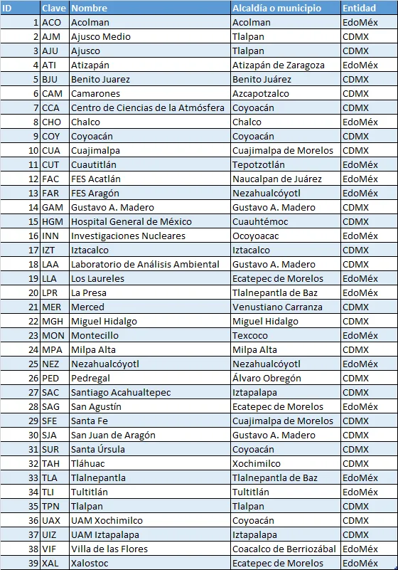
Data on pollutants and meteorological parameters were downloaded from the SIMAT monitoring sites (carbon monoxide -CO-, nitrogen dioxide -NO2-, nitrogen oxides -NOx-, nitric oxide -NO-, ozone -O3-, minor particles at 10 micrometers -PM10-, PM coarse particles that correspond to the difference between PM10 and PM2.5 -PMCO-, particles smaller than 2.52 micrometers -PM2.5-, sulfur dioxide -SO2-, ambient temperature -TMP-, relative humidity -RH-, atmospheric pressure -PA-, barometric pressure -PBa-, wind speed -WSP- and wind direction -WDR-) and a single base was generated. The initial information represents the hourly records of 39 sites (ACO, SUR, TAH, TLA, TLI, SJA, PED, SAG, SFE, TPN, BJU, GAM, LAA, MPA, FAR and SAC) automatic monitoring, however, due to the construction of an air quality monitoring system, not all sites monitor all pollutants and meteorological parameters. In addition to this, in 2017 an earthquake was recorded in Mexico City that damaged the infrastructure of some institutions where monitoring stations were located, which led to the removal of measurement equipment from those places. Another characteristic that this type of phenomena presents is the dependence of its records on time cycles since its behavior is influenced by the time of year and time of day (effect of thermal inversions, rainy season, atmospheric stability, peak hours of the day, location of pollution sources, among others).

Table.1. List of SIMAT air quality monitoring sites.

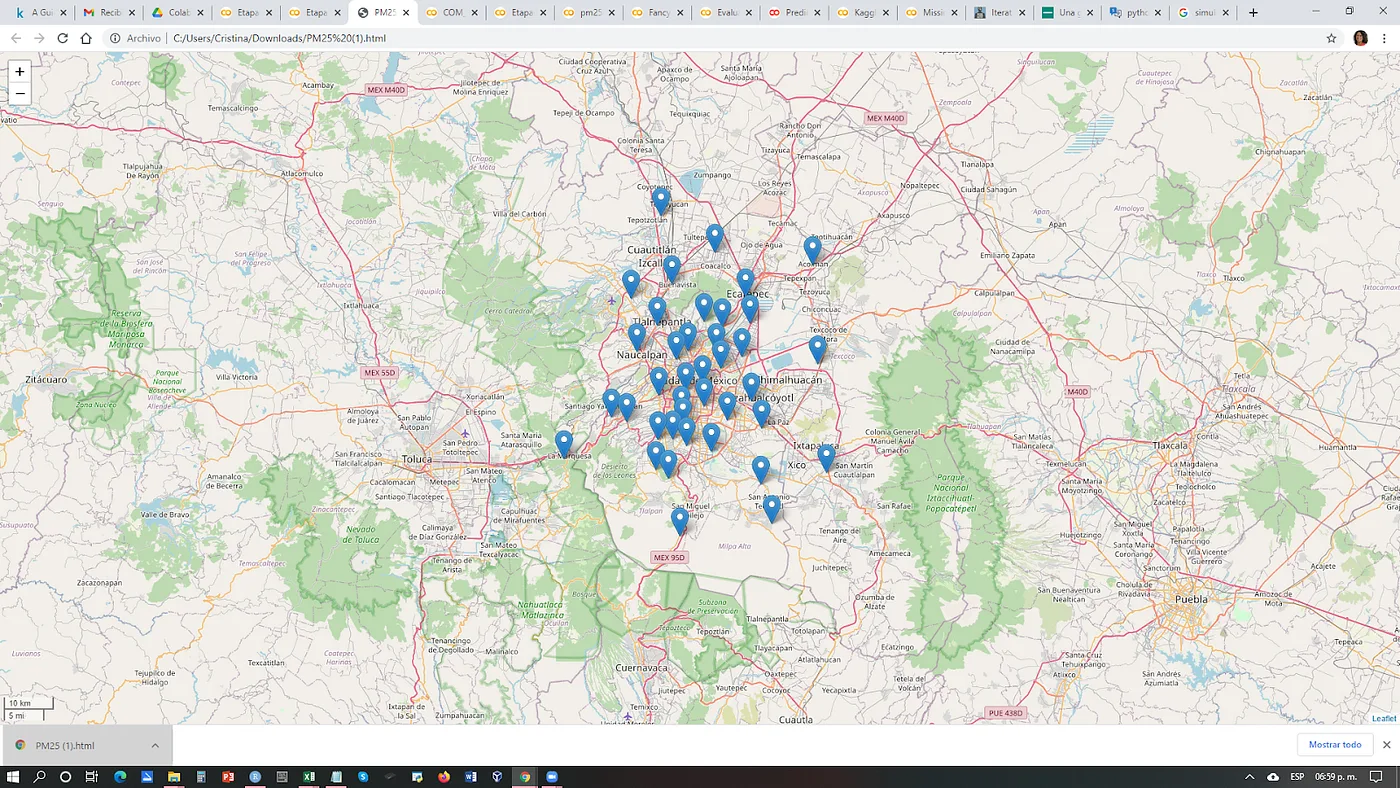
Map 1. Location of SIMAT air quality monitoring sites (2020).

All of this involved several steps being taken to determine the inclusion of sites for this analysis.

Data preprocessing

Site selection:

1. Aquellos que monitorean PM2.5 (a saber: TLA, SJA, PED, SAG, SFE, XAL, CCA, MGH, UAX, UIZ, CAM, COY, MER, NEZ, HGM, AJM, BJU, INN, AJU, GAM, MPA, MON, SAC y FAR)
2. Those who present registrations in 2019 and have at least 75% of registrations from that year (namely: TLA, PED, SFE, XAL, CCA, AJM, MON, MER, HGM, NEZ and GAM).

Map 2. Location of the eleven SIMAT air quality monitoring sites that will be modeled.

The continuous recording of this type of data requires a measurement quality assurance and control program, which implies the loss of records, for example, when calibrations and reviews of the correct operation of automatic equipment are carried out; as well as, due to the lack of electrical energy input that entails the reactivation of the equipment. This is reflected in having missing values (missing values) in the databases, therefore, a treatment must be proposed to fill in missing data.

Exploratory data analysis

1. The sites were explored to identify possible associations between them for each parameter.
2. It was reviewed if there is any dependency with lag in hours for each parameter.
3. The exploration associated with the direction of the wind was carried out to identify any dependence related to the direction from which the wind comes.

For the exploratory analysis, the library was used Open air de r-project.

Filling missing data

1. It is considered to use models that allow adjustment even with missing data in the target or response variable (PM.2.5).
2. Likewise, it is considered to use models that require that the response variable does not contain missing values, so several methods of imputation of missing values for PM2.5 will be used (it should be noted that due to the nature of this type of data, filling in with the mean, median or some other constant is not recommended). Previously, a comparison of the methods will be carried out with a complete data set in which the missing data is simulated and the imputation error is evaluated to select the best missing filling model (the type of missing data that governs this phenomenon is identified (MCAR, MAR or NMAR for its acronym in English), which refer to a completely random behavior, randomly or does not follow a random process, respectively.
3. In the case of time forecast models, it is required that the regressor variables do not have missing values in the training period or the testing period. Furthermore, future data is required for PM2.5 forecasting; therefore, imputation of missing data must also be performed.

For the process of filling in missing data, several techniques were explored without achieving good results since they generated constant values for filling (for example, the options that the routine has implemented Fancyimpute of Python), including:

• SimpleFill: Replaces missing entries with the mean or median of each column.
• KNN: Nearest neighbor imputation via record weighting using the root mean square difference of variables where two rows have observed data.
• SoftImpute: Matrix completion using iterative smooth thresholding of SVD decompositions. Inspired by the SoftImpute package for R, which is based on spectral regularization algorithms for learning large incomplete matrices of Mazumder et al.
• IterativeImputer: A strategy for imputing missing values by modeling each feature with missing values as a function of other features in a round-robin fashion. A stub that links to scikit-learn's IterativeImputer.
• IterativeSVD: Matrix completion using iterative low-rank SVD decomposition. Should be similar to SVDimpute's missing value estimation methods for DNA microarrays. Troyanskaya et. to the.
• MatrixFactorization: Direct factorization of the incomplete matrix in low-rank U and V, with an L1 sparsity penalty on the elements of U and an L2 penalty on the elements of V.
• NuclearNormMinimization - Simple implementation of Exact Matrix Completion via Convex Optimization by Emmanuel Candes and Benjamin Recht using cvxpy. Too slow for large arrays.
• BiScaler: Iterative estimation of row/column mean and standard deviation to obtain a doubly normalized matrix. It's not guaranteed to converge, but it works well in practice. Taken from Matrix Completion and Low-Rank SVD via Fast Alternative Least Squares.

Therefore, it was decided to fill in from the hourly profile of the data series, that is, considering the average of records for the same hour throughout the series, this ensures that there is a differentiated value per hour and constant data is not generated for all the missing records.

Transform the data

On some occasions it is advisable to transform the data to obtain a better fit, however some transformations may cause a lack of interpretation of the results, which is why it is recommended to use simple transformations that are easy to reverse at the time of interpretation.

In the case of the response variable (PM2.5) it will be transformed with the natural logarithm to have better behavior of the data.

Y=ln(PM2.5)

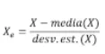
In the case of the regressors (or covariates), the data are standardized in each variable, because each one, by its nature, is in varied units and scales.

Fit models

The bookstore Prophet from facebook (fbprophet), allows forecasting time series data based on an additive model where non-linear trends are adjusted to annual, weekly and daily seasonality, plus the effects of holidays. It works best with time series that have strong seasonal effects and multiple seasons of historical data. Prophet is robust to missing data and trend changes, and typically handles outliers well.

To model the Prophet time series, we separate the signal into the following additive components:

y(t)= g(t) + s(t) + h(t) + εt

Where:

• y(t) is the variable to be predicted
• g(t) is the trend function that models nonperiodic changes using a nonlinear saturation growth model or a piecewise linear regression model. You can configure this using parameters.
• s(t) is the seasonal functional (annual, weekly and daily) that models the periodic changes in the value of the time series. This component is modeled using a Fourier transform and you can add your own seasonalities if you wish.
• h(t) represents the function for modeling holidays and special impact events. You can add your own set of custom holidays and special events.
• εt is the error/noise of models assumed to have a distribution

For a more detailed description of the algorithm consult https://peerj.com/preprints/3190/

The algorithm works best with time series that have strong seasonal effects and multiple seasons of historical data. Prophet is robust to missing data in the output variable and to changes in trend, and typically handles outliers well.

The training and test groups were established to evaluate the models considering the sequence of the information and, unlike taking them at random, it was established to leave the first four years as the training period and the last year as the test period.

Results

Select data

The air quality data from the stations located in the Metropolitan Area of Mexico City were selected, which present records between the years 2015 and 2020, a filter was made from these stations to have the stations that had PM2.5 records, a second filter was made to these stations to have the stations that recorded data in the year 2019 and that had annual sufficiency (at least 75% of hourly records in the year) in this way there was a set of eleven stations (see Map 2).

Exploratory data analysis

The exploratory analysis allowed us to know the behavior of each variable, in the case of PM2.5 (Figure 1) it was observed that there are differences between the stations, since some present a greater number of atypical events, this is mainly due to the place where each station is located and the pollution sources associated with them.

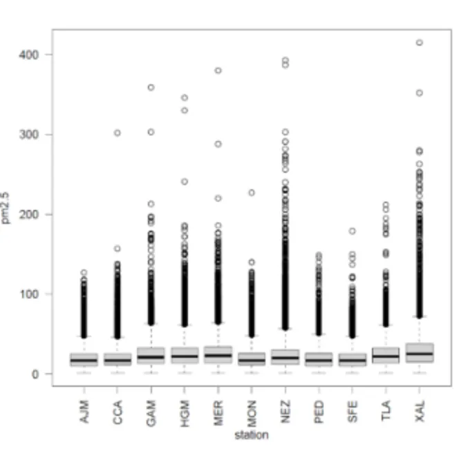
Figure 1. PM2.5 behavior of the eleven sites chosen for modeling

To exemplify the rest of the results, the case of the Ajusco Medio (AJM) station is presented; for its location, see Map 2.

The analysis by variable shows that there are frequent periods of absence of data, the difference in the behavior of each parameter (some have distributions skewed to the right, others to the left and some have a symmetrical distribution, some have more than one mode and there are usually atypical data) (Figure 2).

The behavior of PM2.5 with respect to the direction of the wind shows a clear association in the winter months (January and December) in the northeast direction and with a strip of influence from the north to the east, and in the months of April and May it is repeated with a slight shift towards the south (red colors in Figure 3), the dilution of this pollutant is also identified in the rainy months, since blue, green and yellow colors predominate in all wind directions.

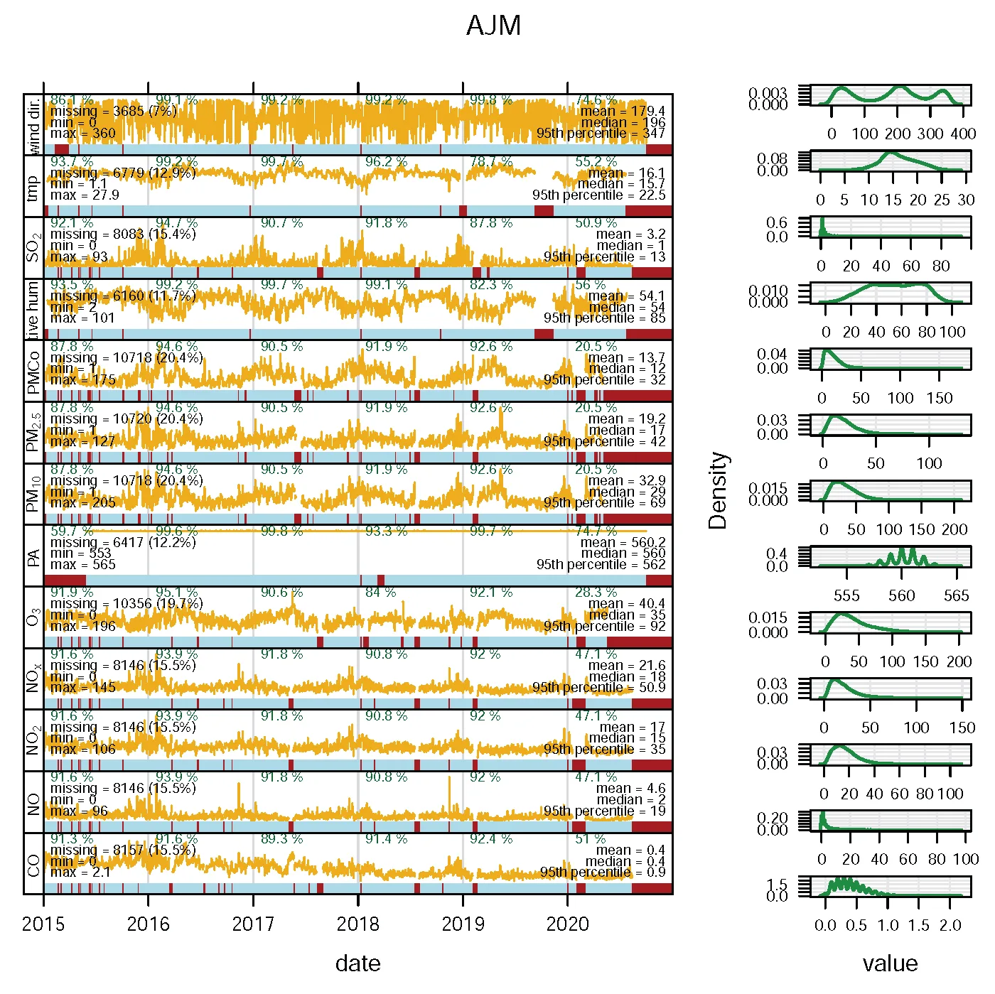
Figure 2. Distribution of hourly records at the Ajusco Medio (AJM) station and representation of the concentration rose disaggregated by month

The disaggregation by climatic season for each year allows us to appreciate the changes throughout the period (it should be noted that the winter season considers December of one year and January and February of the following year), the change from red to orange is identified over the years in the winter season and in 2020 these colors were not recorded (it presents lower concentrations). The influence of spring (March to May) is also marked with high concentrations mainly in 2016, 2017 and 2019 (Figure 4).

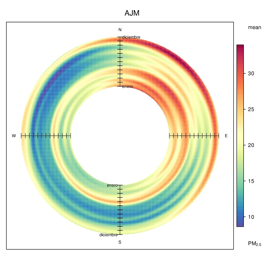
Figure 3. Representation of PM2.5 concentration rose broken down per month

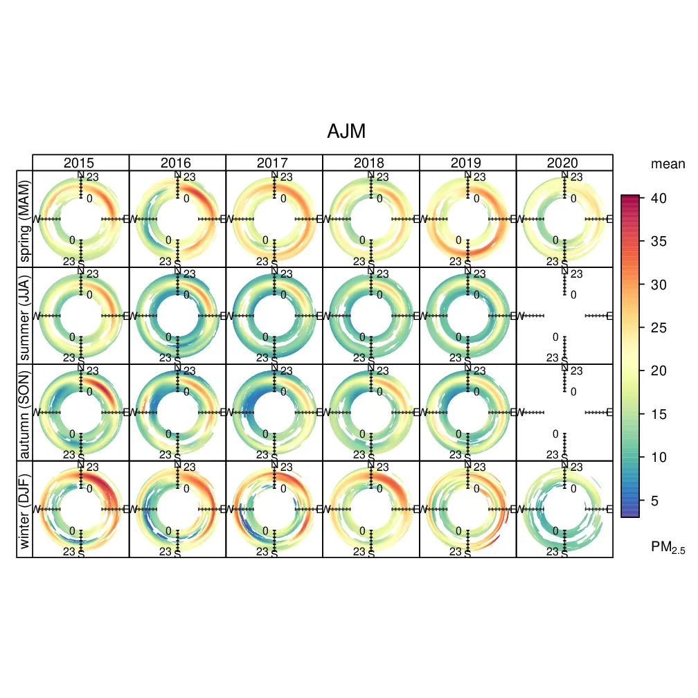
Figure 4. Distribution by climatic season (spring, summer, autumn and winter) of the concentration rose disaggregated by year.

The time series of the hourly PM2.5 records is represented in Figure 5, you can see the blank spaces corresponding to the missing values on those days, as well as the variation of the phenomenon and the extreme values.

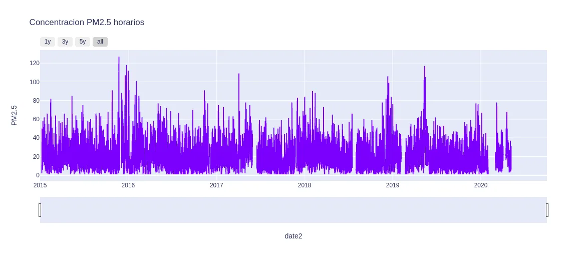
Figure 5. Time series of hourly PM2.5 concentration in the period 2015–2020 for the AJM station.

The modeling will be carried out with daily average PM2.5 records, so their behavior was visualized in Figure 6.

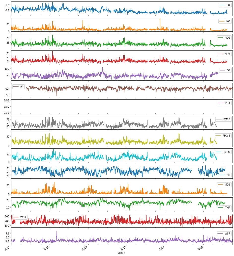
Figure 6. Time series of daily averages for the different pollutants and meteorological parameters in AJM (2015–2020).

The variation of PM2.5 from daily records allows the presence of cycles associated with months and years to be identified (Figure 7).

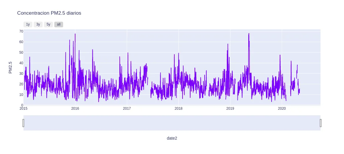
Figure 7. Daily concentration of PM2.5 in the period 2015–2020 for the AJM station.

Transform the data

In the case of PM2.5 the transformation was with the natural logarithm, Figure 8 shows the original behavior and the transformation, where the aim is to have a distribution more in line with symmetry.

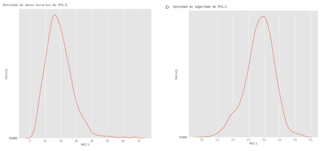
Figure 8. Distribution of PM2.5, original and transformed (AJM, 2015-2020).

In the case of the regressors, the transformation was performed separately for the training and test data set (Figure 9).

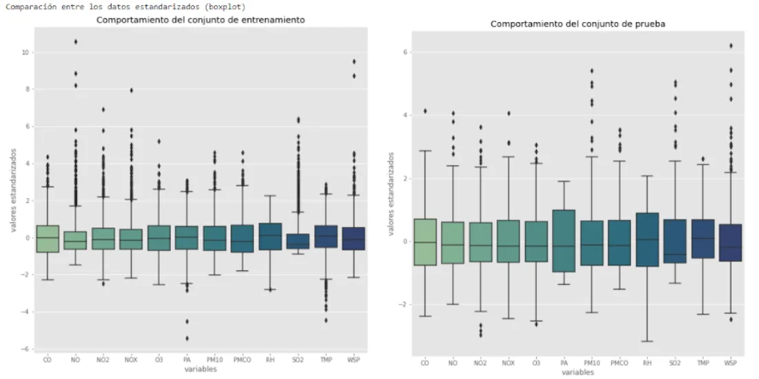
Figure 9. Distribution of standardized regressors in the training and test set (AJM, 2015–2020)

Fit models

We begin by modeling the univariate PM2.5 series without imputing missing values since the model handles the lack of information in the output variable.

We generate the training set from 2015–01–01 until the 2018–12–31 and the test set from 2019–01–01 and until the 2020–09–30 to train and evaluate the model respectively. Mexican holidays are incorporated into the model to achieve a better fit.

Code fragment with the values of the hyperparameters used to train the algorithm:

pro_change=Prophet(changepoint_range=0.9,yearly_seasonality=True,

holidays=holidays)

pro_change.add_country_holidays(country_name=’MX’)

forecast = pro_change.fit(train).predict(future)

fig= pro_change.plot(forecast);

a = add_changepoints_to_plot(fig.gca(), pro_change, forecast)

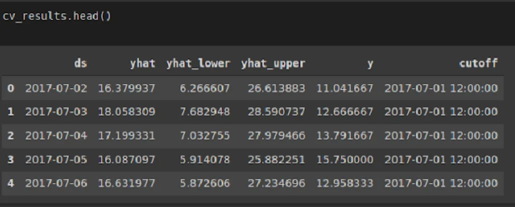
The model generates a predictive value called yhat, and a confidence interval with lower limit yhat_lower and upper limit yhat_upper for the PM2.5 concentration, we set the confidence level of 95%.

Code fragment to do cross validation

from fbprophet.diagnostics import cross_validation

cv_results = cross_validation( model = pro_change, initial = ‘731 days’, horizon = ‘365 days’)

In Figure 10, the black dots represent the average daily PM2.5 concentration values, the dark blue curve is the prognosis generated by the model and the celestial blue zone is the 95% confidence interval.

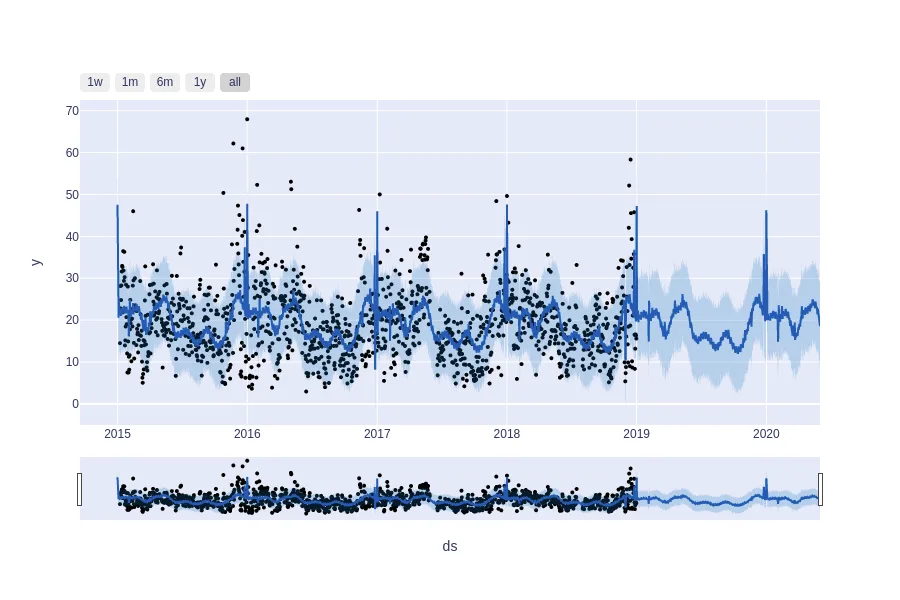
Figure 10. PM2.5 model adjustment at the AJM station

Figure 11 shows the decomposition of the series into its trend, holidays, weekly and annual seasonality.

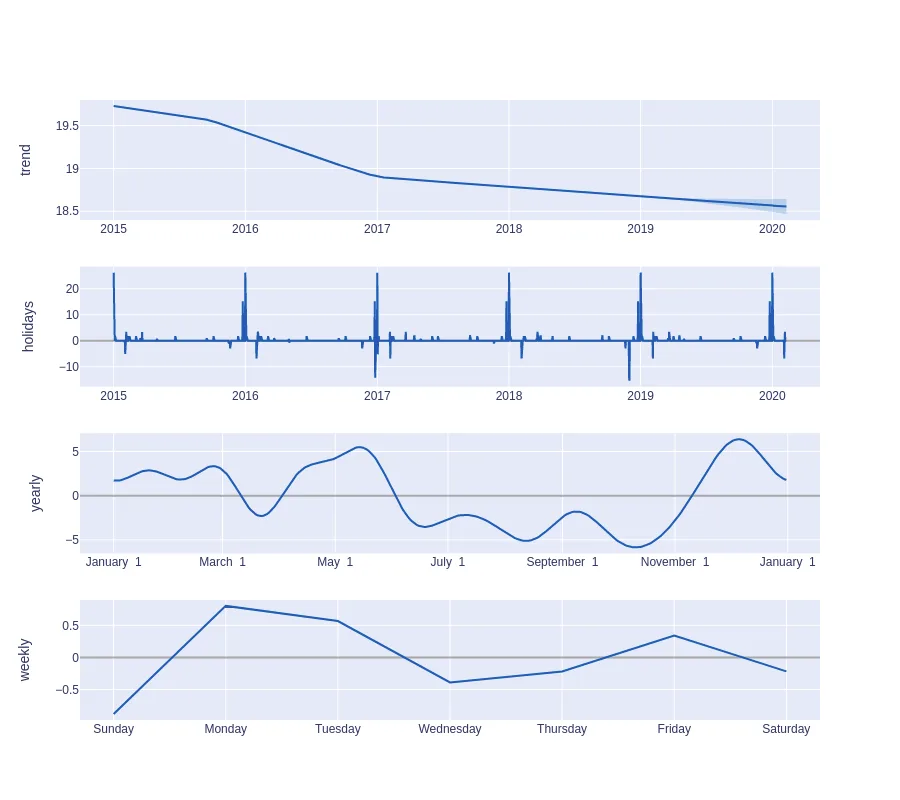
Figure 11. Discomposition of the PM2.5 series at the AJM station.

The function performance_metrics can be used to calculate some useful statistics to measure prediction performance (yhat, yhat_lower and yhat_upper versus y), as a function of distance from the boundary (how far into the future the prediction was). The calculated statistics are Mean Squared Error (MSE), Root Mean Squared Error (RMSE), Mean Absolute Error (MAE), Mean Absolute Percentage Error (MAPE), Mean Absolute Percentage Error (MDAPE), and Estimate Coverage. yhat_lower and yhat_upper. These are calculated in a moving window of the predictions in the dataframe after sorting by horizon (ds minus cutoff). By default, 10% of the predictions will be included in each window, but this can be changed with the argument rolling_window.

Code fragment to obtain metrics

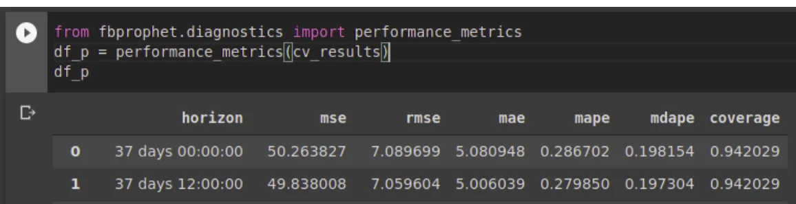
Once the different models were run, the metrics were compared to determine the best model. In the case of AJM, the best model from RMSE was the fit with hyperparameters, followed by the model with general regressors. For all metrics, the model with the lowest error was the hyperparameters model.

Table 2. Comparison of the metrics of the adjusted models (AJM, 2015–2020)

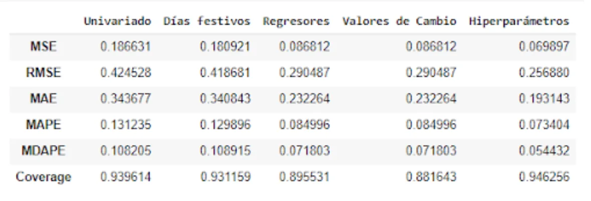
Below is the graphical representation of the best fitted model, distinguishing the training period, the test period and the forecast (Figure 12).

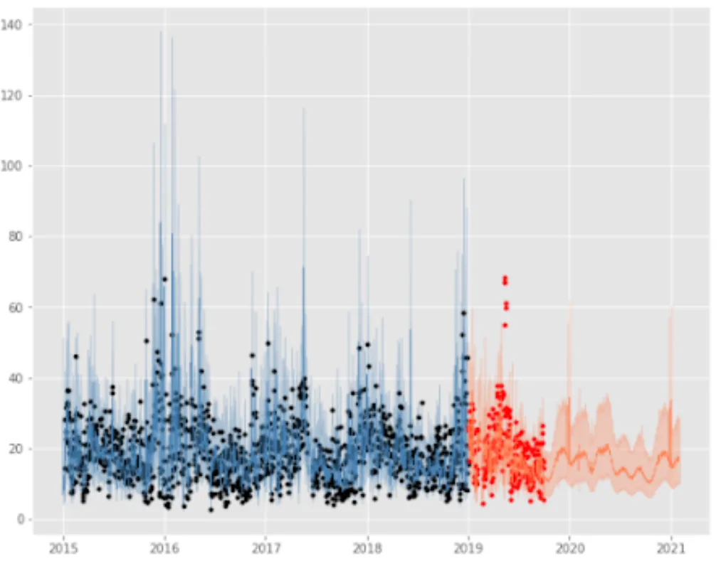
Figure 12. Fit of the best model (AJM, 2015-2020)

As an added result when modeling this data, we can detect if any health risk may occur in future days, with reference to the World Health Organization Guidelines for the 24-hour average of PM2.5 (25 g/m³) and the ranges established in the Mexican AIR and HEALTH Index (NOM-172-SEMARNAT-2019).

Table 3. Air quality risk levels (2020)

Source: Environmental Commission of the Megalopolis (CAMe)

In the case of Ajusco Medio, the forecast identifies possible records between the good and acceptable air quality bands, and when considering the confidence interval of the model (Figure 13), it is identified that the records could reach the bad air quality band, which could present some risk to the population.

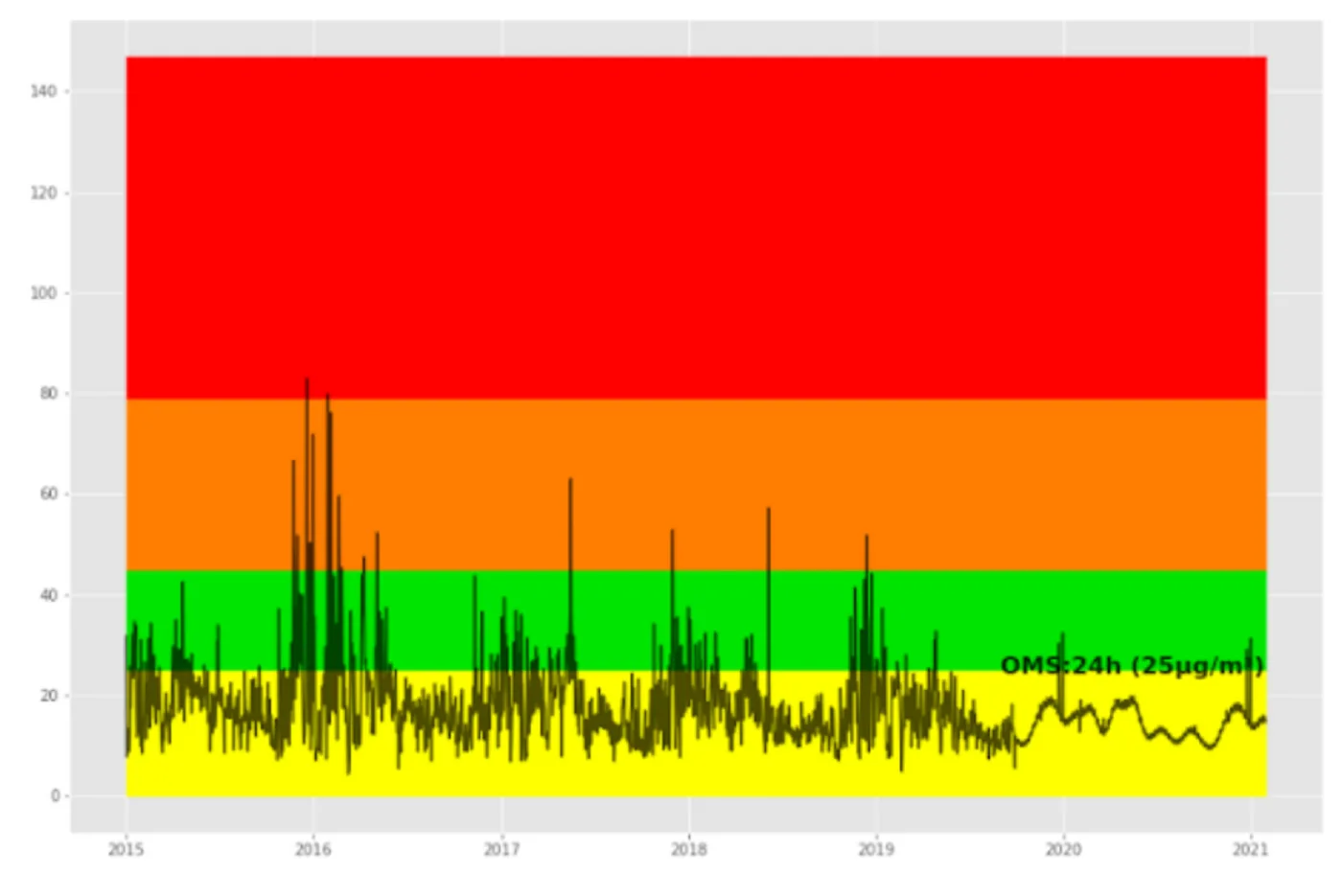
Figure 13. Air quality alerts in AJM, measured data and forecast as of 01/31/2021

What's next

A sea of opportunities opens up to improve this first approach to modeling air quality through artificial intelligence. The models were applied to each of the stations, but a multiseries model can be developed. In the same way, the total number of variables against which the adjustment was carried out was established, but a search can be carried out among the regressors that present the greatest contribution to the PM2.5 modeling.

Develop an application to disseminate the results.

Try other data sets from different cities.

and much more...

References

Basheer O, et al. Imputation of Missing Values in Daily Wind Speed Data Using Hybrid AR-ANN Method Modern Applied Science 9(11):1, June 2015

Mazumder R., Hastie T., Tibshirani R. Spectral regularization algorithms for learning large incomplete matrices. The Journal of Machine Learning Research 11, 2287–2322

Medina F. and Galván M. Data imputation: theory and practice. ECLAC, 2007.

Shaadan N. and RahimN A M. 2019 J. Phys.: Conf. Ser. 1366 012107.

Taylor SJ, Letham B. 2017. Forecasting at scale. PeerJ Preprints 5:e3190v2

Troyanskaya G, et al. Missing Value Estimation Methods for DNA Microarrays June 2001. Bioinformatics 17(6):520–525

WHO, 2016. Health risk assessment of air pollution — general principles. Copenhagen: WHO Regional Office for Europe; 2016.

Libraries or packages

Carslaw, D. C. and K. Ropkins, (2012) openair — — an R package for air quality data analysis. Environmental Modelling & Software. Volume 27–28, 52–61.

Facebook Open Source, Prophet. https://facebook.github.io/prophet/

Fancyimpute https://github.com/iskandr/fancyimpute

Members

• Cristina Ortuño Mojica
• Luis Rafael Diaz
• Carolina Trujillo
• Gabriel Coello

Project presentation: DemoDay

Open video or resource

Repository

In the following repository you will find the code used to develop that application: https://github.com/SaturdaysAI/Projects/tree/master/LATAM\_remote/SaturdaysAI-LATAM\_AIreySalud\_2020-main

More Artificial Intelligence!

The mission of Saturdays.ai is to make artificial intelligence more accessible (#ai4all) through intensive courses and programs where projects for good are carried out (#ai4good).

Explore our AI master’s programme at https://saturdays.ai/master-ia-online/

If you want to learn more about artificial intelligence join our community at community.saturdays.ai or visit us on our website www.saturdays.ai Join us!